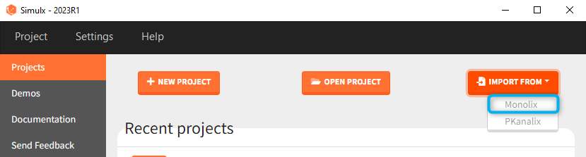
There are three methods to start a project in Simulx: create a new project, open an existing project and import a project from Monolix or PKanalix. To import a project from Monolix is as simple as clicking on the button “Import from Monolix” in the Simulx home tab. It is the easiest way to build a simulation scenario, because everything to run a simulation is prepared automatically. As a result, it saves a lot of time.You can always modify current simulation elements, define new ones and change the scenario, so the flexibility of Simulx is not compromised.
1. Simulx project structure with “Import from Monolix”
2. A typical simulation workflow with a project imported from Monolix
Simulx project structure
Importing a project from Monolix creates a Simulx project with pre-defined elements. You can use them to re-simulate the dataset from the Monolix project or as a base for a new simulation scenario. These elements appear in the Definition tab:
- Model, population parameters and individual parameters estimates and output variables are imported from Monolix.
- Occasions, covariates, treatments and regressors are imported from the dataset (used in the imported Monolix project).
Simulx sets default exploration and simulation scenarios – they are ready to run. They contain one exploration group to simulate a typical individual (in the exploration tab) and one simulation group to re-simulate the Monolix project (in the simulation tab).
Default simulation elements
- model: mlxtran model with blocks [INDIVIDUAL], [COVARIATE] and [LONGITUDINAL].
- pop.params.:
- mlx_PopInit [no POP.PARAM task results]: (vector) initial values of the population parameters from Monolix.
- mlx_Pop: (vector) population parameters estimated by Monolix.
- mlx_PopUncertainSA (resp. mlx_PopUncertainLin): (matrix) an element which enables to sample population parameters using the covariance matrix of the estimates computed by Monolix if the Standard Error task (Estimation of the Fisher Information matrix) was performed by stochastic approximation (resp. by linearization). To sample several population parameter sets, this element needs to be used with replicates.
- indiv.params.:
- mlx_IndivInit [no POP.PARAM task results]: (vector) initial values of the population parameters from Monolix.
- mlx_PopIndiv: (vector) population parameters estimated by Monolix.
- mlx_PopIndivCov: (table) population parameters with the impact of the covariates used in the model (but no random effects).
- mlx_EBEs: (table) EBEs (conditional mode) estimated by Monolix.
- mlx_CondMean: (table) conditional mean estimated by Monolix.
- mlx_CondDistSample: (table) one sample of the conditional distribution (first replicate in Monolix).
- covariates [if used in the model]:
- mlx_Cov: (table) ids and covariates read from the dataset.
- mlx_CovDist: (distribution) distribution of covariates from the dataset with empirical mean and variance for continuous covariates, set as lognormal for positive continuous covariates, normal for continuous covariate with some negative values, and multinomial low based on frequencies of modalities for categorical covariates.
- treatment:
- mlx_AdmID: (table) ids, amounts and dosing times (+ tinf/rate or washouts) read from the dataset for each administration type.
- outputs:
- mlx_observationName: (table) ids and measurement times read from the dataset for each output of the observation model
- mlx_predictionName: (vector) uniform time grid with 250 points on the same time interval as the observations for each continuous output of the structural model.
- mlx_TableName: (vector) uniform time grid with 250 points on the same time interval as the observations for each variable of the structural model defined as table in the OUTPUT block.
- occasions:
- mlx_Occ [if used in the model]: (table) ids, times and occ(s) read from the dataset.
- regressors:
- mlx_Reg [if used in the model]: (table) ids, times and regressor values and names read from the dataset.
Default exploration and simulation scenarios
Exploration:
- Indiv.params: mlx_IndivInit or mlx_PopIndiv.
- Treatment: one exploration group with mlx_AdmId for all administration IDs.
- Output: mlx_predictionName for all predictions defined in the model.
Simulation:
- Size: number of individuals read from the dataset.
- Parameters: mlx_PopInit or mlx_Pop.
- Treatment: mlx_AdmId for all administration IDs.
- Output: mlx_observationName for all observations.
- Covariates: mlx_cov if used in the model.
- Regressor: mlx_reg if used in the model.
Interface allows to have an overview on all defined elements, modify them and create new ones as well as build simulation scenarios. But, if you modify the imported model, then Simulx will remove all simulation elements. In addition, if you remove occasions, then all occasion-dependent simulation elements will be removed as well.
A typical simulation workflow with a project imported from Monolix
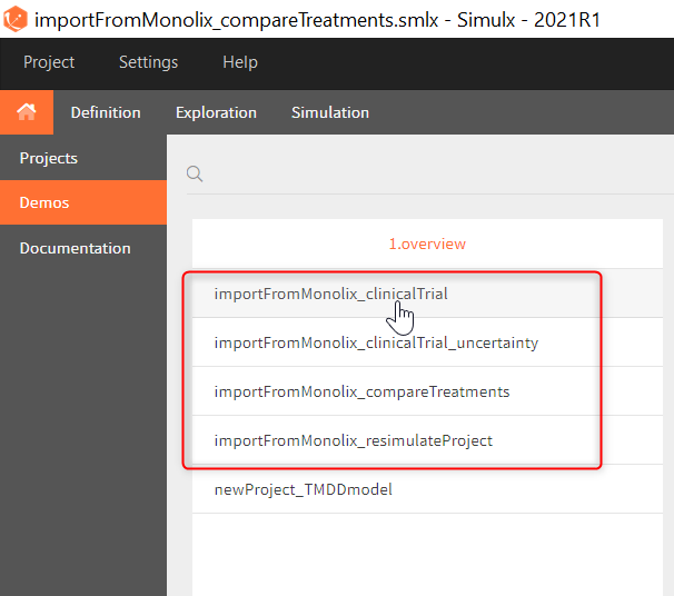
The projects shown here are available as demo projects in the interface “1.overview – importFromMonolix_xxx.smlx”:
This example is based on a PK-PD model for Warfarin developed and estimated in Monolix. The Warfarin dataset contains concentration and PCA(%) measurements for 32 individuals, who received different oral doses of the drug. Firstly, the goal of the Simulx project is to use the information from the Monolix project to test the efficacy and safety conditions for different treatments. Secondly, to simulate clinical trials and compare various dosing regimens strategies. Simulations should answer the following questions:
- Which “loading dose” strategy assures a rapid steady state without a concentration peak?
- Do multi-dose treatments meet the efficacy and safety criteria?
- What is the uncertainty of the percentage of individuals in a target due to the variability between individuals and due to the size of a trial group?
Model:
The PK model includes an administration with a first order absorption and a lag time. It has one compartment and a linear elimination. The PD model is an indirect turnover model with inhibition of the production. All individual parameters have log-normal distribution besides the Imax parameter, which is logitNormally distributed. In addition, the log-transformed scaled weight covariate explains intra-individual variability of the volume, age covariate has an effect on the clearance and sex covariate on the baseline response. Finally, the combined-1 error model is used in the observation model of the concentration, and the constant model of the response.
0. Re-simulation of the Monolix project
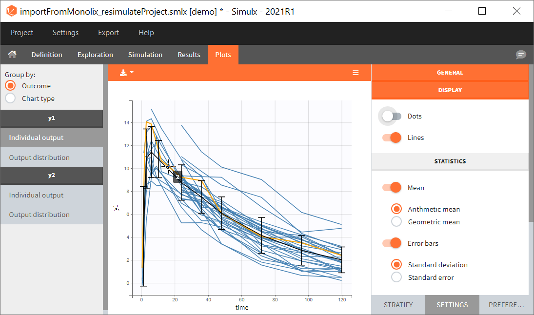
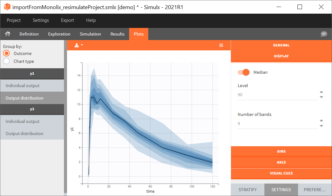
[Demo project “1.overview – importFromMonolix_resimulateProject.smlx”]
You can download the Monolix project for this example, here. To import it in SImulx, first unzip the folder, then start a Simulx session, click on “Import from: Monolix” and browse the .mlxtran file. After importing a project from Monolix, the task buttons “simulation” and “run” in the Simulation tab re-simulate the project. Plots and results are generated automatically. Results are tables for outputs and individual parameters and plots display model observations as individual outputs and distributions.
1. Exploration of the loading dose strategies
[Demo project “1.overview – importFromMonolix_compareTreatments.smlx”]
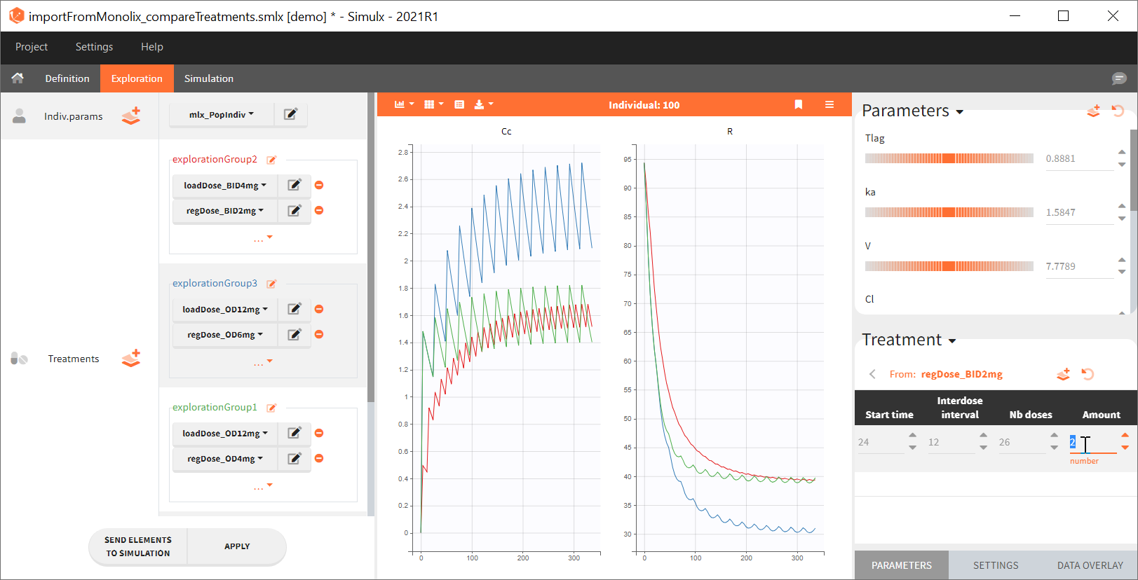
Exploration tab simulates a typical individual. After importing a project from Monolix (the same as in the previous example), you can choose different types of individual parameters elements, eg. equal to population parameters estimated by Monolix or EBEs. Using several exploration groups allows to compare different treatments in one chart. The goal of this example is to test how many days of a “loading dose” are necessary to reach a steady state without a peak of the concentration. Starting dosing regimens are:
- 1 day with a load dose 12mg OD followed by 13 days with a 6mg single dose OD
- 1 day with a load dose 12mg OD followed by 13 days with a 4mg single dose OD
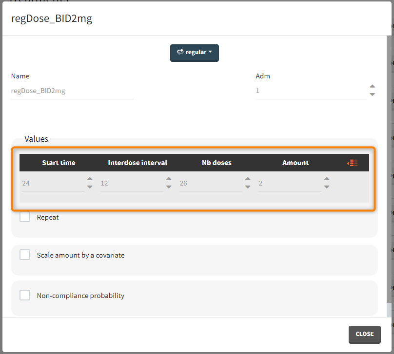
- 1 day with load doses 4mg twice a day (BID) followed by 26 doses of 2mg every 12 hours.
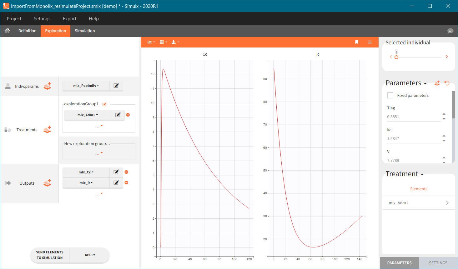
“Loading dose” treatments elements are of manual type (with time of a dose and amount), while multi-dose elements are of regular type. Regular type includes a specification of a treatment period, inter-dose interval and number of doses. You combine treatments elements directly in the exploration tab (in the left panel).
Output is the concentration prediction Cc and the response prediction R on a regular time grid over the whole treatment period (t = 0:1:336) . The plot displays one subplot per output, and all exploration groups (=dosing regimen) together on each subplot. In the right panel, you can edit treatment elements and parameters interactively – predictions are updated on-the-fly for all groups to help you find which exact regimen is the most promising.
2. Treatment comparison: percentage of individuals in the target
[Demo project “1.overview – importFromMonolix_compareTreatments.smlx”]
Simulation scenario
Exploration tab performed simulation on one individual. In the simulation tab, Simulx simulates a population of individuals. SImulation outputs can be further post-processed to calculate, for example, the percentage of individuals in the target for different treatment arms. This simulation scenario uses the following treatment and output elements.
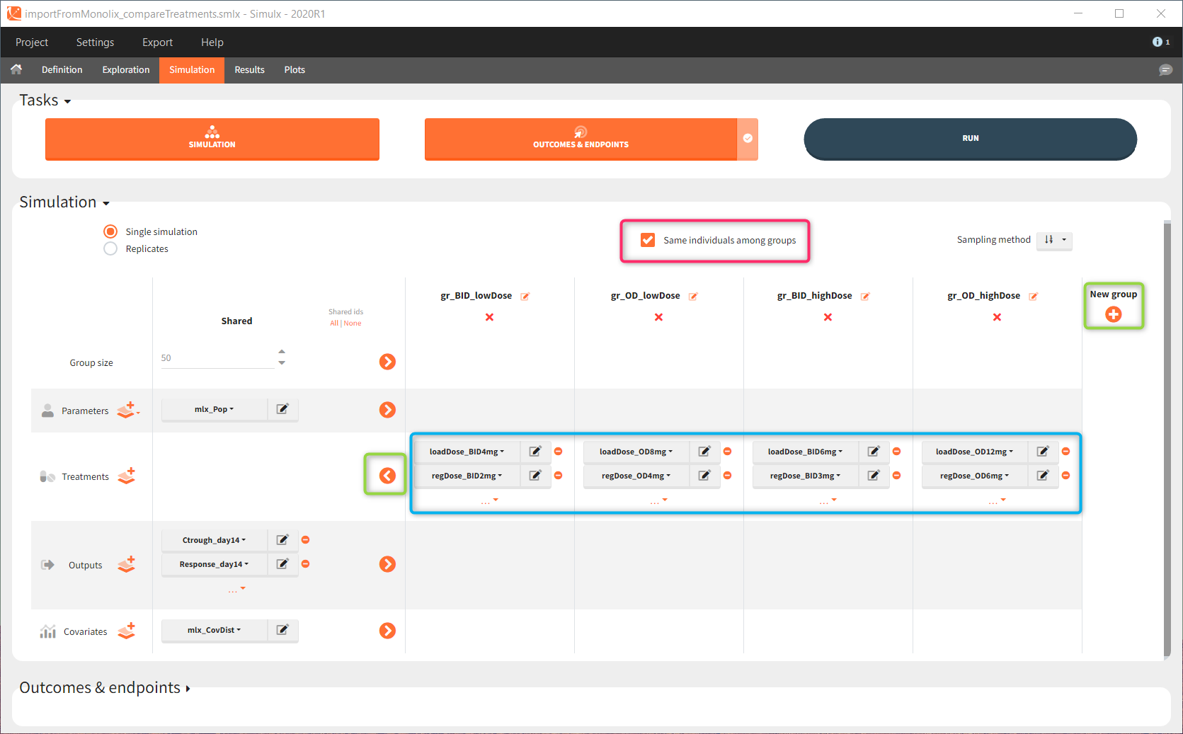
- BID treatment: One day of a “loading dose” with 4mg or 6mg dose twice a day (BID), followed by 26 doses of 2mg or 3 mg respectively each 12 hours.
- OD treatment: One day of a “loading dose” with 8mg or 12mg dose once a day (OD), followed by 13 doses of 4mg or 6 mg respectively each 24 hours.
- Outputs: manual type using model predictions (Cc and R) at time equal 336h.
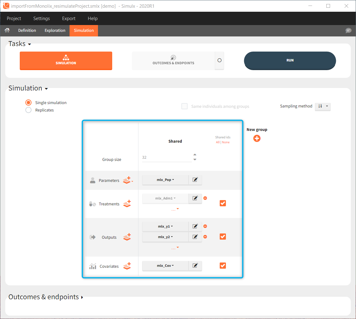
In the simulation tab, the button “plus” adds a new group and “arrows” (green frames below) move elements from the shared section to the group specific section. For treatment, each group has a specific combination of treatments (blue frame). In addition, the option “same individuals among groups” removes the effect of intra-individual variability between individuals (red frame). As a consequence, the observed differences between groups are only due to the treatment and simulation can use a smaller number of individuals.
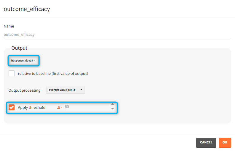
The comparison between groups is in terms of the percentage of individuals in the efficacy and safety target:
- Efficacy: PCA at the end of the treatment should be less than 60%.
- Safety: Ctrough on the last treatment day should be less than 2ug/mL.
You can calculate it in the outcomes&endpoints section of the simulation tab. Definition of new outcomes includes selecting an output computed in the simulation scenario and post-processing methods. When you apply threshold condition, then outcome is of a binary (true/false) type.
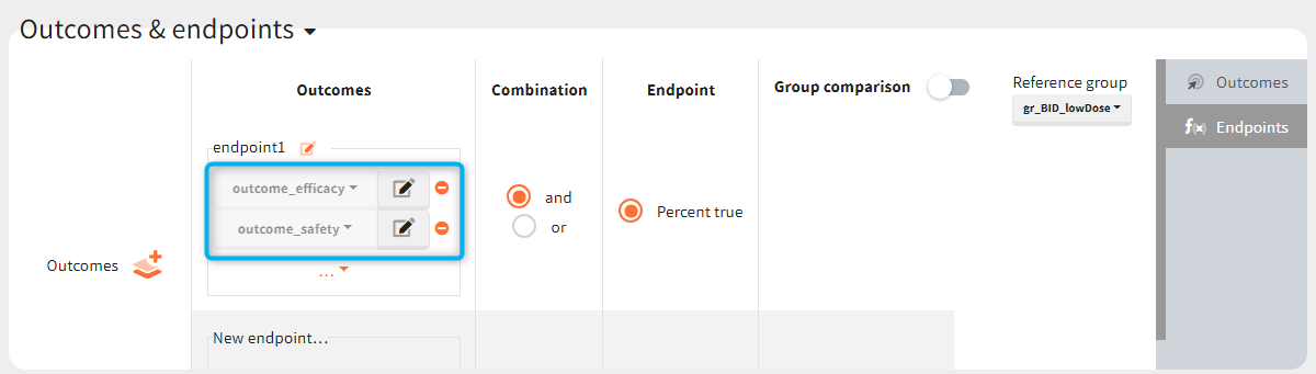
In addition, outcomes can be combined together (blue frame below), and an endpoint summarizes “true” outcomes over all individuals in groups.
Analysis
Similarly to the task button “Simulation”, which runs the simulation, the “Outcomes & endpoint” button performs post-processing, which in this example means calculating the efficacy and safety criteria and the number of individuals in the target. When you run this task, SImulx generates automatically the results in the “endpoint” section and plots for outcomes distributions.
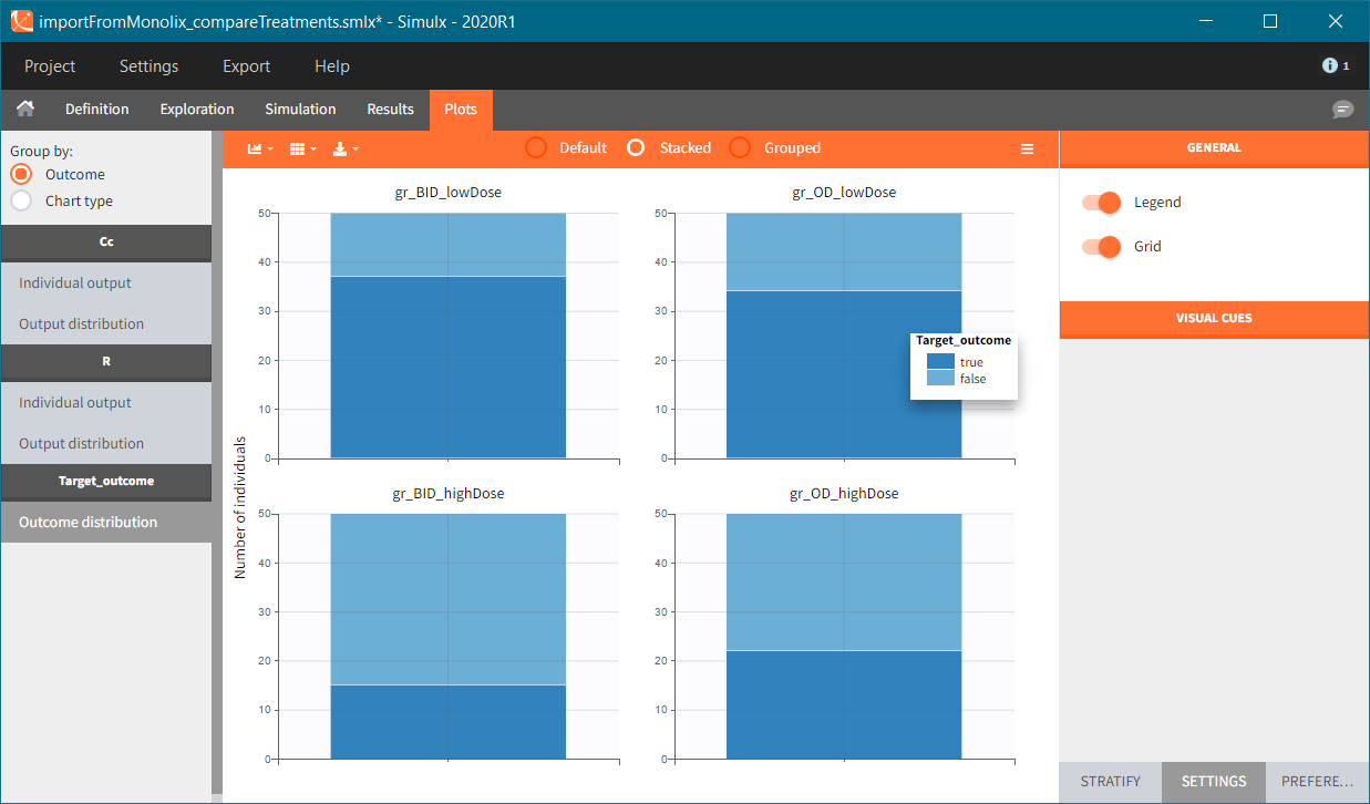
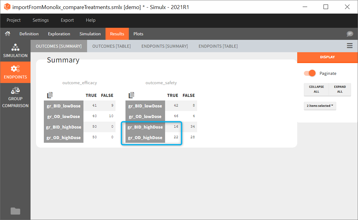
In this example, the outcome distribution compares the number of individuals in the target between groups. The highest number of “true” outcomes is in the group with the low level dose twice a day (gr_BID_lowDose). Failure to satisfy the safety criteria by the two groups with the high dose level causes large numbers of “false” outcomes. In fact, the endpoint results show that for these two groups less than half of the individuals have Ctrough below the safety threshold (blue frame below).
3. Clinical trial simulation and uncertainty of the results
[Demo project “1.overview – importFromMonolix_clinicalTrial.smlx”]
The previous step shows that the high dose level violates the safety criteria in more than 50% of individuals. Therefore, the simulation of a clinical trial uses only one dose level with the BID and OD administration.
The goal is to analyse the effect of the uncertainty due to the variability between individuals, measurement errors and number of individuals in a trial.
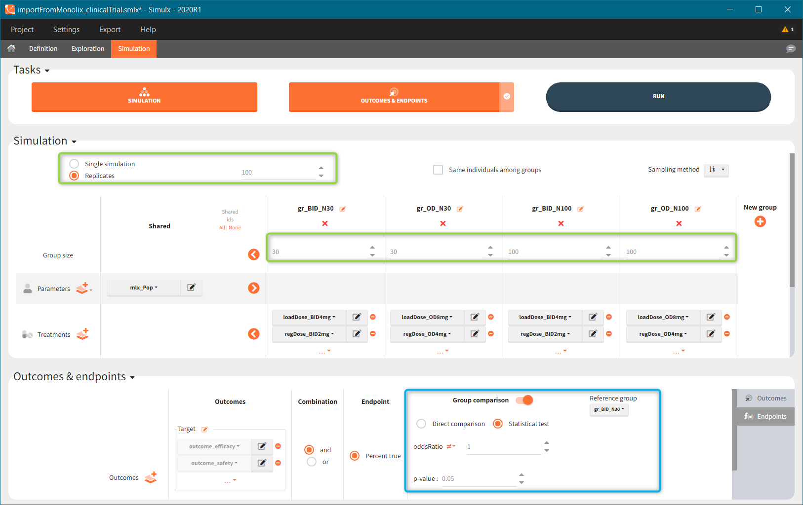
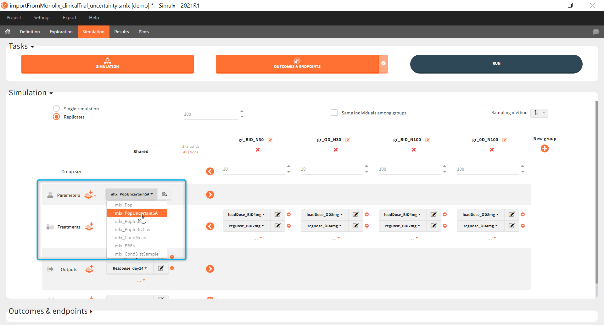
New simulation scenario has four groups which combine different dosing regimens (BID or OD) with different group sizes (30 or 100). Outputs are model observations at the end of the treatment. To simulates the scenario several times (green frames), use the option “replicates”. As a result, the endpoints summarize the outcomes not only over the groups but also over the replicates.
[Starting from the demo project “1.overview – compareTreatments.smlx”, change number of replicates to 100, and add two groups: one with treatment as for GR_BID, other as GR_OD. Move “number of ids” as group specific, and set N=30 for one BID-OD pair and N=100 for the other. Change names to indicate group sizes.]
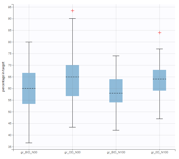
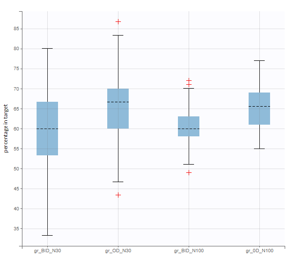
After running both tasks, plots display the endpoint distribution as a box plot with the mean value (dashed line) and standard deviations for each group. As expected, the uncertainty is lower for trial with more individuals. However, the mean values remain at similar levels.
“Group comparison” option in the Outcomes&endpoints section compares the endpoints values across groups (blue frame). Selecting different reference groups and hypothesis (through the odds ratio) allows to change the objectives. Moreover, calculation of new outcomes or endpoints do not require re-running a simulation because the post-processing is a separate task.
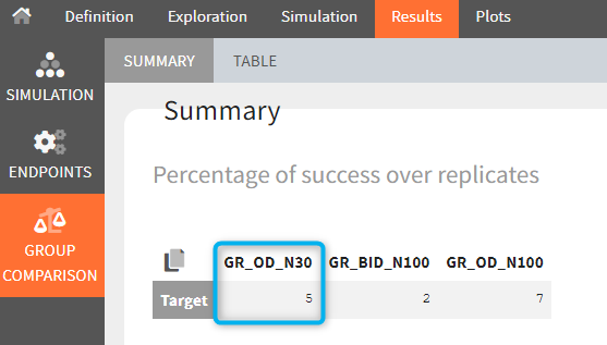
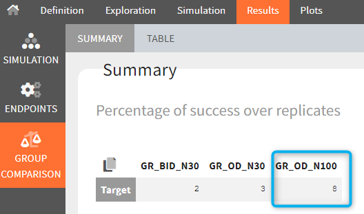
The statistical test checks if any of the dosing regimens, BID or OD, is better than the other. Firstly, in the smaller trial so the gr_BID_N30 group is the reference and the hypothesis states that the odds ratio is different from one. For each replicate, if the p-value is lower than selected 0.05, then a test group (GR_OD_N30) is a “success”. Results summary in the “group comparison” section shows that only 5% of the test group replicates are successful (upper image below), which suggests that OD dosing regimen is not significantly better than BID. Larger trial size might give different results. Change reference group to gr_BID_N100 and re-run the outcomes & endpoints task. Percentage of successful replicates for gr_OD_N100 is higher, 8%, (lower image below), but it is comparable to the previous result.
4. Propagation of parameter uncertainty to the predictions
[Demo project in 2021 version only “1.overview – importFromMonolix_clinicalTrial_uncertainty.smlx”]
In the previous step, we replicated the study 100 times to check the impact of sampling different individuals on the endpoint, and on the power of the study. For all these replicates, we sampled individuals using the same population parameters (so same typical values and deviations of random effects).
The goal of this final step is to check the impact of the uncertainty of population parameter estimates on the final endpoint and study power. For this, starting from the 2021 version, it is possible to use the population parameter element mlx_PopUncertainSA (resp. mlx_PopUncertainLin) if standard errors have been computed by stochastic approximation in the original Monolix project (resp. by linearization). Now the 100 replicates will be samples using each time different population parameter values, which are sampled from the variance-covariance matrix of the estimates imported from Monolix.
When running again simulation and outcomes with this population parameter element, we obtain a higher uncertainty on the endpoint than in step 3, since now we observe in addition the uncertainty related to the estimation of parameters in Monolix.