Definition of regressors elements is available only if the mlxtran model used in a Simulx project uses it. In this case, specification of regressors is mandatory. All regressors used in a model are displayed in one element as separate columns.
Regressors names
- If a Monolix project was imported, then regressors names come from a dataset – headers of columns tagged as regressor.
- When building a project from scratch, regressor names are equal to names used in a model.
Demo projects: 3.6.regressors
Create new regressors element
There are three types of regressor elements:
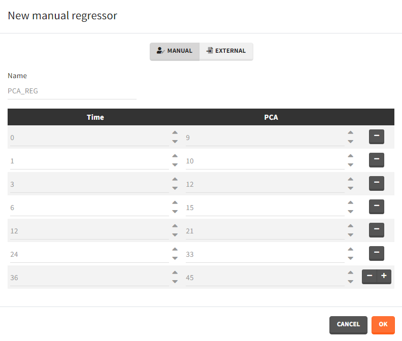
- Manual: It is a vector with manually defined time points and values, which are common for all individuals.
Example: parameter – covariate relationship with the covariate as a regressor
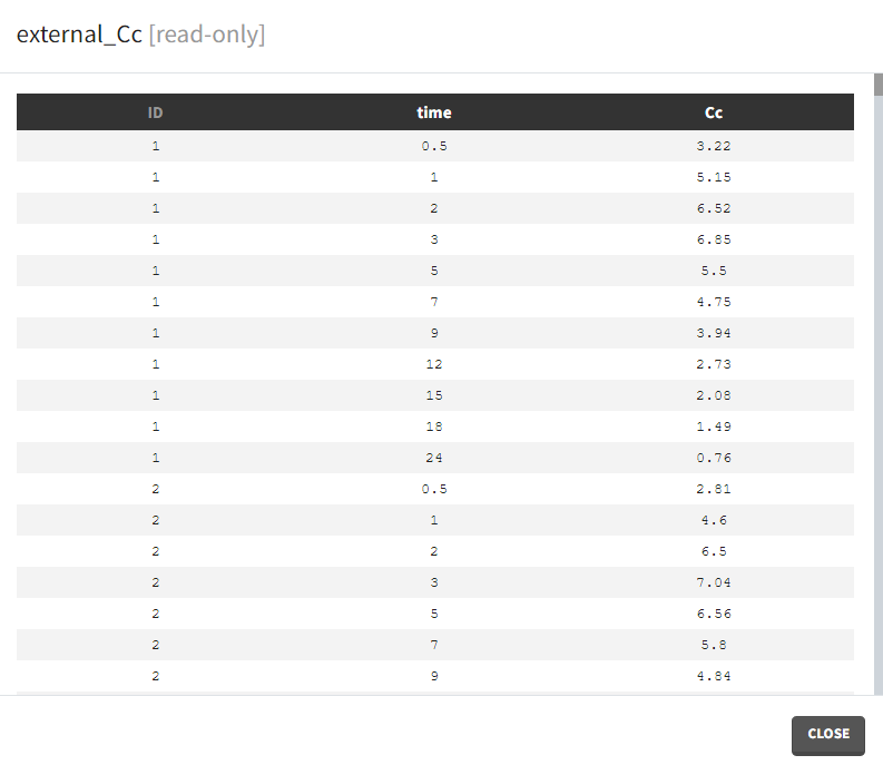
- External: Regressors definition is a table with the following mandatory columns: “time” for time points and “regressor_name” for regressor values. Optionally, it can have a column “id”. In the absence of the “id” column, the time grid is equal for all individuals and occasions (if defined in the model).
Example: PK-PD model with PK measurements as a regressor
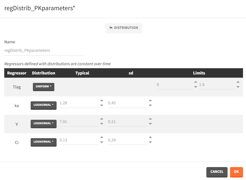
- Distribution: The regressors are described via distribution laws which define their value across individuals. When a distribution is used, the regressor is considered as constant over time. When used in the simulation, new regressor values are sampled from the defined distributions for each individual. The distribution for each regressor can be normal, lognormal or logitnormal with a mean and sd, or uniform with a lower and an upper and bound. If the distribution is lognormal or logitnormal, sd is the standard deviation of the distribution in the Gaussian space, i.e \(V_{reg}=V_{typical}\times exp(\eta)\) with \(\eta \sim N(0,sd^2)\). The typical value is the median of the distribution.
Defining a regressor element as a distribution is convenient for sequential PD model where individual PK parameters have been defined as regressors. After exporting the project to Simulx, new individual PK parameters can be sampled by defining the regressor element for the individual PK parameters as a distribution. Note that correlation terms are not possible.
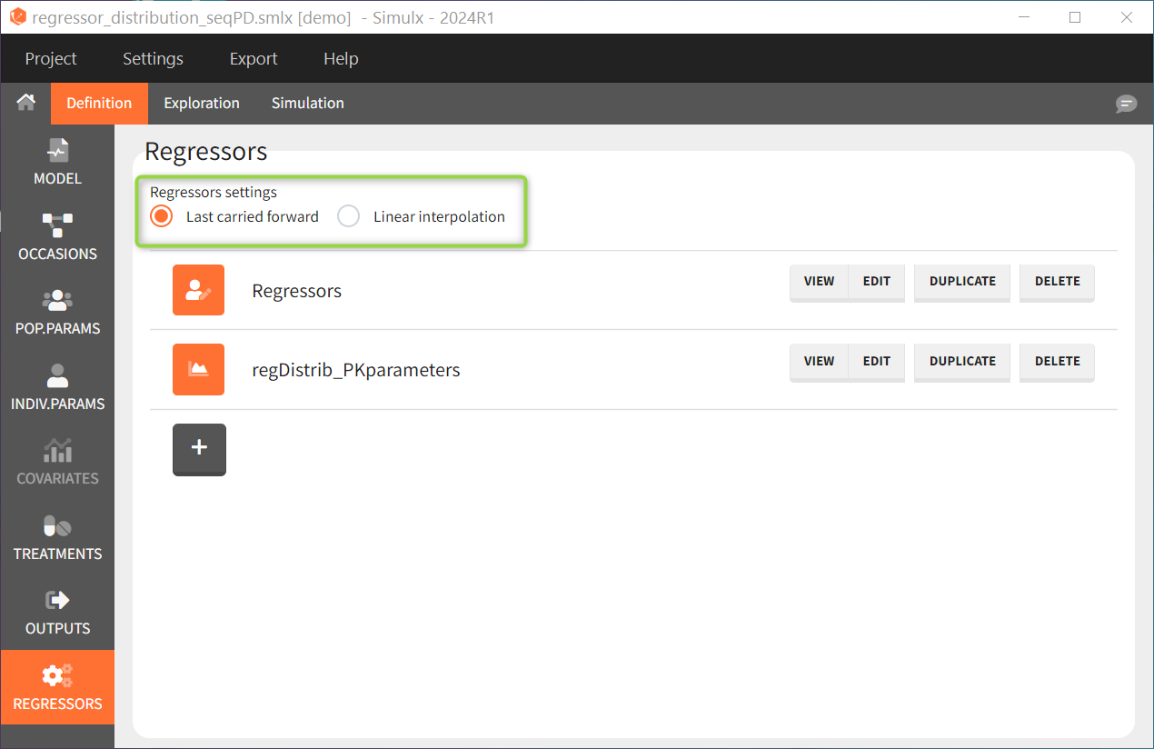
Interpolation between defined values
Regressors are defined over time for a finite number of time points. In between those time points, the regressor value can be interpolated in two different ways:
- last value carried forward: if we have defined \(reg_A\) at time \(t_A\) and \(reg_B\) at time \(t_B\)
- for \(t\le t_A\), \(reg(t)=reg_A\) [first defined value is used]
- for \(t_A\le t<t_B\), \(reg(t)=reg_A\) [previous value is used]
- for \(t>t_B\), \(reg(t)=reg_B\) [previous value is used]
- linear interpolation:
- for \(t\le t_A\), \(reg(t)=reg_A\) [first defined value is used]
- for \(t_A\le t<t_B\), \(reg(t)=reg_A+(t-t_A)\frac{(reg_B-reg_A)}{(t_B-t_A)}\) [linear interpolation is used]
- for \(t>t_B\), \(reg(t)=reg_B\) [previous value is used]
This can be chosen in the DEFINITION > REGRESSORS tab and applies to all defined regressor elements.
Regressors imported from Monolix
Importing a Monolix project generates automatically regressors element with regressors names from the dataset:
- mlx_Reg: contains Ids, times and regressors values read from the dataset. Occasions are included if any.
- mlx_RegDist: (created only if all regressors of each subject and each occasion are constant over time) element of type “distribution” with typical values, standard deviations and probabilities calculated on the individuals of the Monolix project. No correlation between the regressors is assumed. Regressors having only strictly positive values in the Monolix dataset are assumed to follow a log-normal distribution, and the others are set with a normal distribution.
