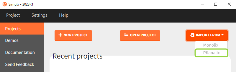
There are three methods to start a project in Simulx: create a new project, open an existing project and from Monolix to Simulx or import project from PKanalix. To import a project from PKanalix, simply click the “Import from PKanalix” option of the “Import from” in the Simulx Home tab. It is the most convenient way to create a simulation scenario, as everything is automatically prepared for running a simulation.You can modify current simulation elements, define new ones and change the scenario at any time, such that the flexibility of Simulx is not compromised.
1. Simulx project structure with “Import from PKanalix”
2. A typical simulation workflow with a project imported from PKanalix
Simulx project structure
Importing a project from PKanalix creates a Simulx project with pre-defined elements. You can use them to re-simulate the dataset from the PKanalix project or as a base for a new simulation scenario. These elements appear in the Definition tab:
- Model, individual parameters estimates and output variables are imported from PKanalix.
- Occasions, treatments and regressors are imported from the dataset.
Moreover, exploration and simulation scenarios are set and ready to run. They contain one exploration group to simulate a typical individual (in the exploration tab) and one simulation group to re-simulate the PKanalix project (in the simulation tab).
Default simulation elements
- model: same structural model as in the CA Model tab of PKanalix. Model is written in mlxtran language
- Indiv.params.:
- pkx_IndivInit [no POP.PARAM task results]: (vector) individual parameters corresponding to the initial values of the parameters in PKanalix
- pkx_Indiv: (table) individual parameters estimated by CA task
- pkx_IndivGeoMean: (vector) geometric mean of individual parameters over all subjects
-
- pkx_AdmID: (table) ids, amounts and dosing times (+ tinf/rate or washouts) read from the dataset for each administration type.
- outputs:
- pkx_ outputName_ FineGrid (vector): for each continuous output of the structural model, a vector with a uniform time grid with 250 points on the same time interval as the observations.
- pkx_ outputName_OriginalTimes (table): for each output of the model, a table with values for ids and observation times corresponding to the measurements read from the dataset
- pkx_TableName: (vector) for each variable of the structural model defined as table in the OUTPUT block, a vector with a uniform time grid with 250 points on the same time interval as the observations.
- occasions:
- pkx_Occ [if used in the model]: (table) ids, times and occ(s) read from the dataset.
- regressors:
- pkx_Reg [if used in the model]: (table) ids, times and regressor values and names read from the dataset.
Default exploration and simulation scenarios
Exploration:
- Indiv.params: pkx_Indiv or pkx_IndivInit.
- Treatment: one exploration group with pkx_AdmId for all administration IDs.
- Output: pkx_outputName_FineGrid for all predictions defined in the model on a fine time grid.
Simulation:
- Size: number of individuals read from the dataset.
- Parameters: pkx_Indiv or pkx_IndivInit.
- Treatment: mlx_AdmId for all administration IDs.
- Output: pkx_outputName_OriginalTimes for all model outputs.
- Regressor: pkx_reg if used in the model.
 Interface allows to have an overview on all defined elements, modify them and create new ones as well as build simulation scenarios. But, if you modify the imported model, then Simulx will remove all simulation elements. In addition, if you remove occasions, then all occasion-dependent simulation elements will be removed as well.
A typical simulation workflow with a project imported from PKanalix
The projects shown here are available as demo projects in the interface “1.overview – importFromPKanalix_xxx.smlx”: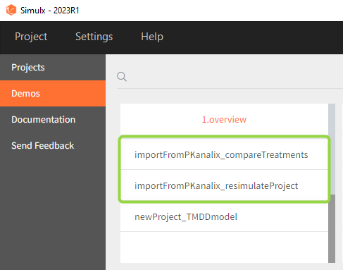
This example is based on a PK-PD model for Warfarin developed and estimated in Monolix. The Warfarin dataset contains concentration and PCA(%) measurements for 32 individuals, who received different oral doses of the drug with the amount 1.5mg/kg. Both the PKPD model and the PKPD parameter estimates come from the compartment analysis (CA) performed in PKanalix. The aim of the Simulx project is to to use the information from the PKanalix project to test the efficacy and safety conditions for different treatments. Possible questions to answer with simulations:
- Which “loading dose” strategy assures a rapid steady state without a concentration peak?
- Do multi-dose treatments meet the efficacy and safety criteria?
Model:
The PK model includes an administration with a first order absorption and a lag time. It has one compartment and a linear elimination. The PD model is an indirect turnover model with inhibition of the production.
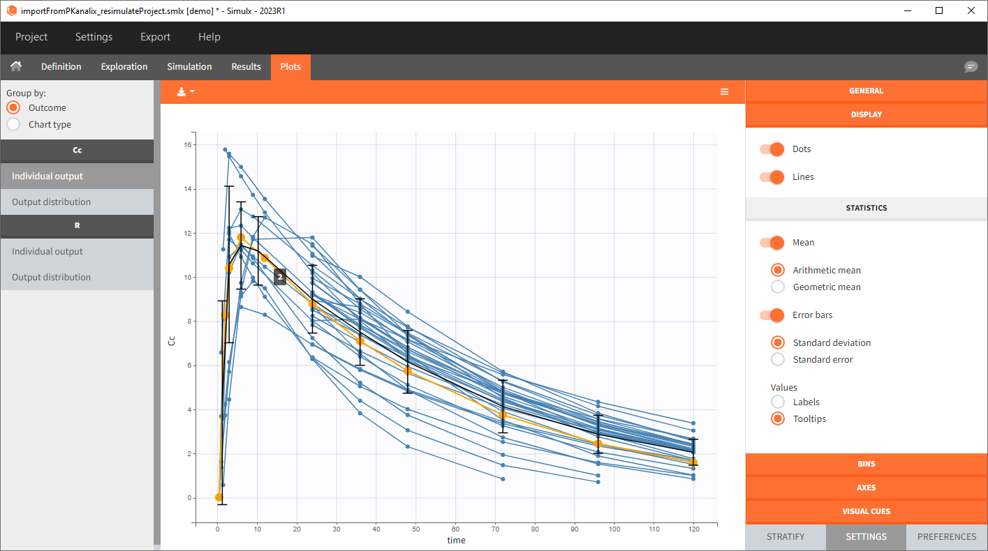
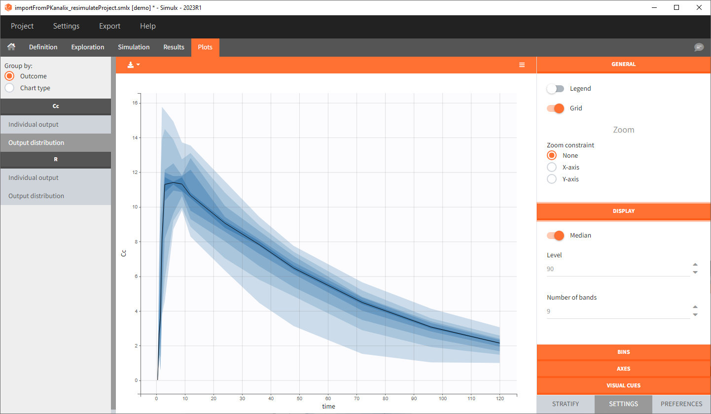
0. Re-simulation of the PKanalix project
[Demo project “1.overview – importFromPKanalix_resimulateProject.smlx”]
You can download the PKanalix project for this example, here. To import it in Simulx, first unzip the folder, then start a Simulx session, click on “Import from: PKanalix” and browse the .pkx file. After importing a project from PKanalix, the task buttons “simulation” and “run” in the Simulation tab re-simulate the project. Plots and results are generated automatically. Results are tables for outputs and individual parameters and plots display model observations as individual outputs and distributions.
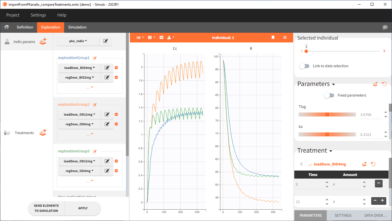
1. Exploration of the loading dose strategies
[Demo project “1.overview – importFromPKanalix_compareTreatments.smlx”]
Definition
The Exploration tab simulates a typical individual. After importing a project (the same as in the previous example), you can choose different types of individual parameters elements, eg. individual parameters estimated in the CA task or geometric mean estimated over all individual parameters. Using several exploration groups allows to compare different treatments in one chart. The goal of this example is to test how many days of a “loading dose” are necessary to reach a steady state without a peak of the concentration. Starting dosing regimens are:
- 1 day with a load dose 12mg OD followed by 13 days with a 6mg single dose OD
- 1 day with a load dose 12mg OD followed by 13 days with a 4mg single dose OD
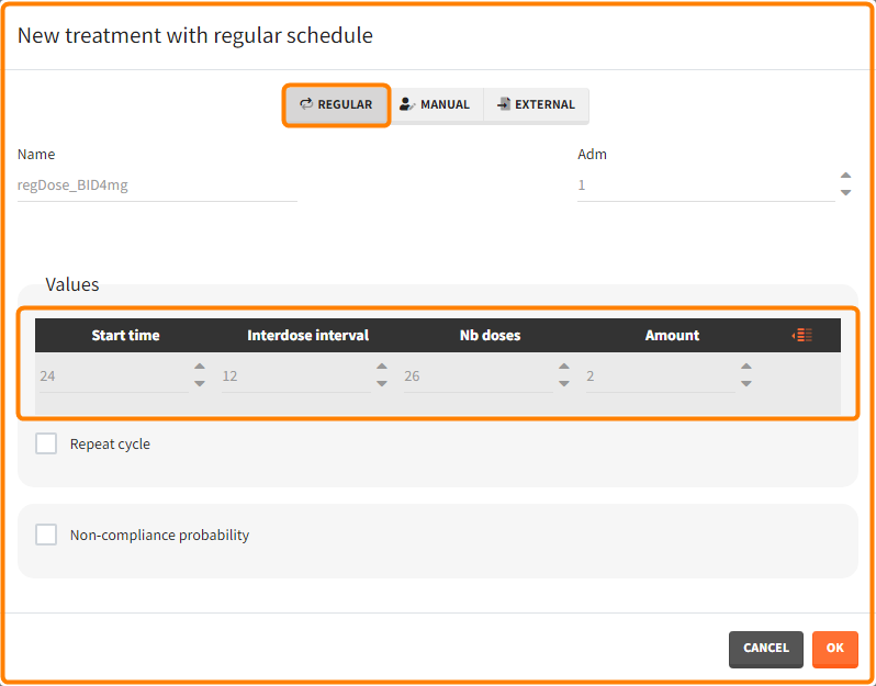
- 1 day with load doses 4mg twice a day (BID) followed by 26 doses of 2mg every 12 hours.
“Loading dose” treatments elements are of manual type (with time of a dose and amount), while multi-dose elements are of regular type. Regular type includes a specification of a treatment period, inter-dose interval and number of doses. You combine treatments elements directly in the exploration tab (in the left panel).
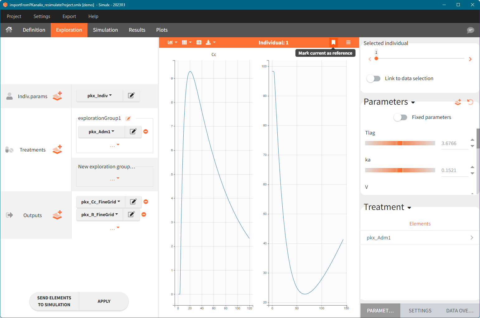
Exploration
Output is the concentration prediction Cc and the response prediction R on a regular time grid over the whole treatment period (t = 0:1:336) . The plot displays one subplot per output, and all exploration groups (=dosing regimen) together on each subplot. In the right panel, you can edit treatment elements and parameters interactively – predictions are updated on-the-fly for all groups to help you find which exact regimen is the most promising.
2. Treatment comparison: percentage of individuals in the target
[Demo project “1.overview – importFromPKanalix_compareTreatments.smlx”]
Simulation scenario
Exploration tab performed simulation on one individual. In the simulation tab, Simulx simulates a population of individuals – in this case all individuals from the original dataset used in the imported PKanalix project. Simulation outputs can be further post-processed to calculate, for example, the percentage of individuals in the target for different treatment arms. This simulation scenario uses the following treatment and output elements.
- BID treatment: One day of a “loading dose” with 4mg or 6mg dose twice a day (BID), followed by 26 doses of 2mg or 3 mg respectively each 12 hours.
- OD treatment: One day of a “loading dose” with 8mg or 12mg dose once a day (OD), followed by 13 doses of 4mg or 6 mg respectively each 24 hours.
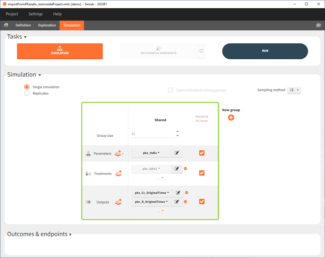
- Outputs: regular type using model predictions (Cc and R) up to time 336h.

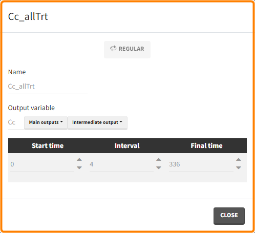
The Simulation tab consists of the same element blocks as the Exploration tab. the button “plus” adds a new group and “arrows” (green frames below) move elements from the shared section to the group specific section. For treatment, each group has a specific combination of treatments (orange frame). As output a new vector was defined. Click on the “edit” icon to see the time discretization. Both output vectors, for the concentration as well as for the response range from time point 0 to time point 336 with step size 4 (unit is in hours h).
The option “Same individual among groups” removes the effect of intra-individual variability between individuals (red frame). As a consequence, the observed differences between groups are only due to the treatment itself. This case
Outcomes & endpoints
The efficacy and safety criteria correspond to the following conditions:
- Efficacy: at the end of the treatment PCA should not exceed 60%.
- Safety: on the last treatment day concentration should not exceed 1.5µg/mL
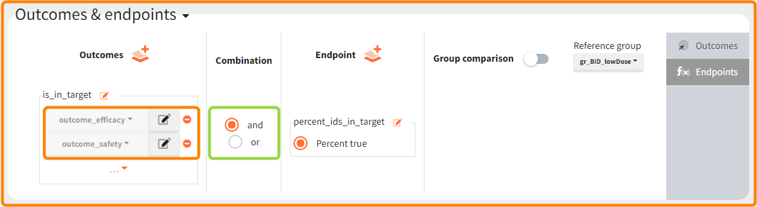
You can calculate it in the outcomes&endpoints section of the simulation tab. Definition of new outcomes includes selecting an output computed in the simulation scenario and post-processing methods. When you apply threshold condition, then outcome is of a binary (true/false) type.

In addition, the defined outcomes can be combined together with a logical operator (green frames below), and an endpoint summarizes “true” outcomes over all individuals in groups.
Analysis
Analogous to the “Simulation” button that runs the simulation, the ” Outcomes & Endpoint” button performs the post-processing – calculates the efficacy and safety criteria and the number of people in the target. In addition, the execution of this task automatically generates the results in the “Endpoint” section and graphs for the outcomes distributions.
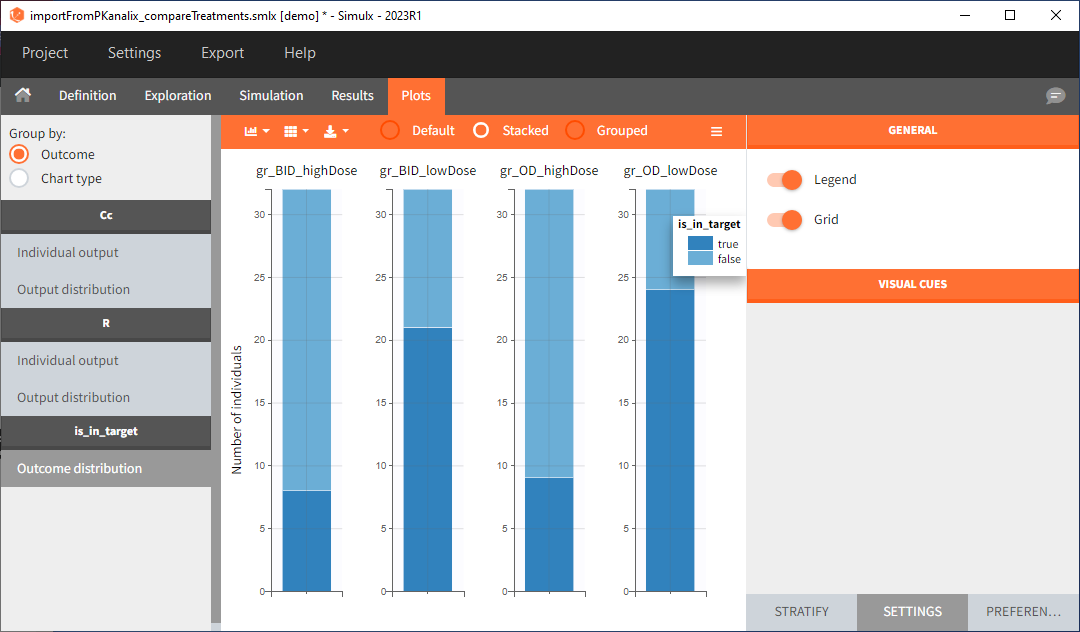
In this example, the outcome distribution compares the number of individuals in the target between treatment groups. Stack charts show the highest number of ” true ” results (\(\widehat{=}\) at time t=336h PCA \(\le\) 60% AND Cc \(\le\) 1.5µg/mL) in the group with the low dose once daily (gr_OD_lowDose).
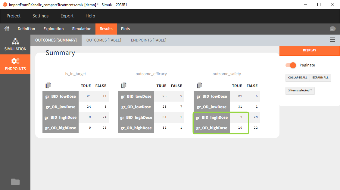
Large number of “false” in the two groups with the high doses (gr_OD_highDose, gr_BID_highDose) relates to the violation of the safety criteria. The endpoint results show that for these two groups, less than 1/3 of the subjects have concentration below the safety threshold (green frame below).
Conclusion
In the higher multi-dose regimens, although 31 of 32 subjects reach the efficacy criterion, only 9 to 10 of these subjects meet the safety criterion.
The group with the lower dose administered once per day, gr_OD_lowDose, have the highest success rate: 24 out of 32 subjects, i.e. 75% of the subjects meet both the safety and the efficacy criteria.
Go to typical simulation workflow with a project imported from Monolix, to see how you can extend this analysis to simulations of clinical trials and assessment of the uncertainty.
