Outcomes, endpoints group comparison are in a dedicated section “Outcomes&endpoints” of the Simulation tab.
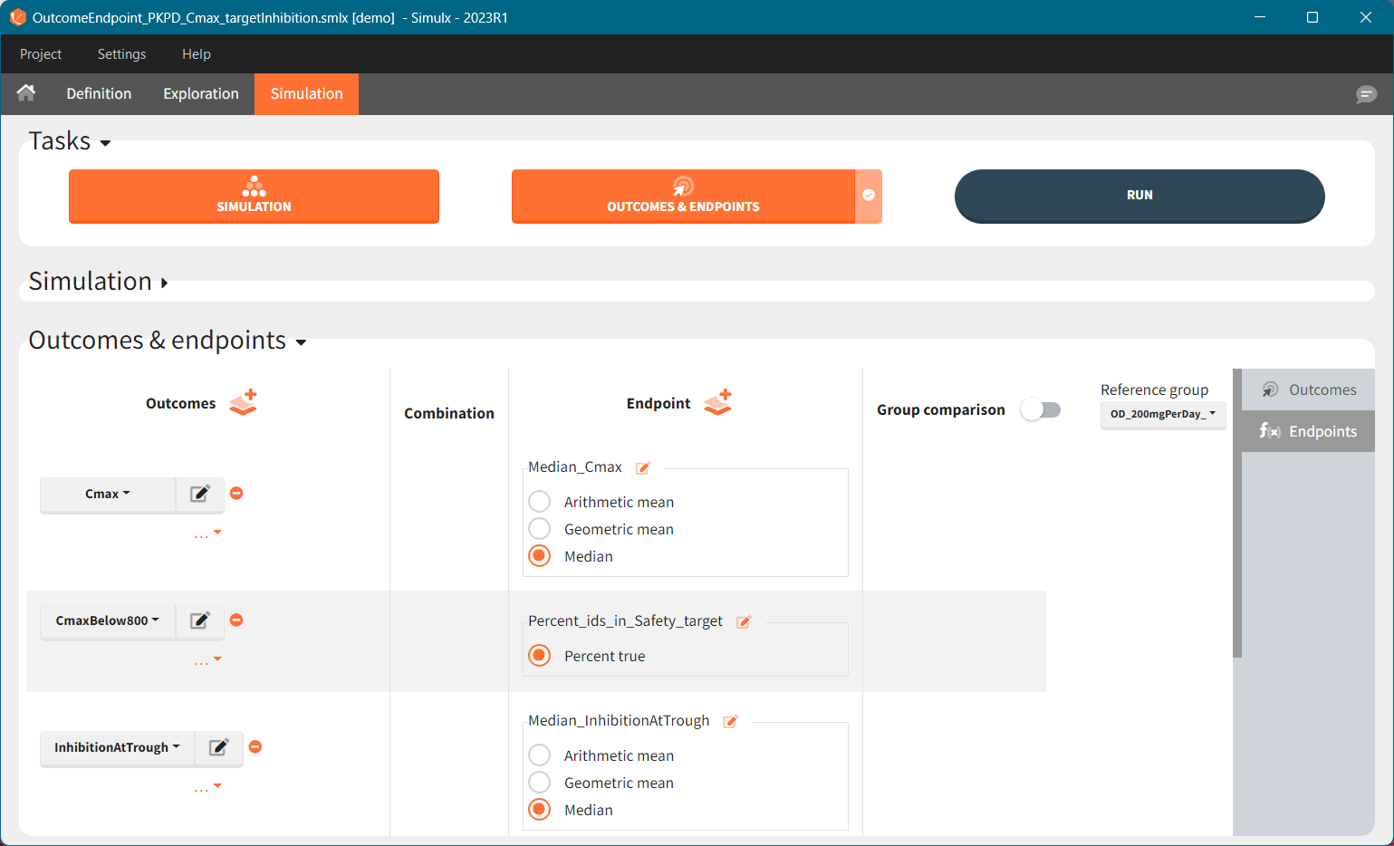
To calculate outcomes and endpoints click on the “Outcomes&Endpoints” button in the Tasks section (on top). The outcomes are a post-processing of the simulation outputs, so remember that you have to first run the “Simulation” task. You can also selected the task “Outcomes&Endpoints” in a scenario (circle radio button on the right hand side of the task button) and click the button RUN – Simulx will run both tasks automatically one by one.
The calculated values are displayed in the Results tab and Plots tab.
Outcomes
Outcomes represent a post-processing of the simulation outputs done for each individual. They correspond to the measure of interest per individual. Outcomes have different types: values (e.g Cmax), binary true/false (e.g true if Cmax < threshold), or time-to-event (e.g time to NADIR).
To create a new outcome, click on the “plus” button next to Outcomes header or on the “+ New outcome element” within the list of outcomes for an endpoint:
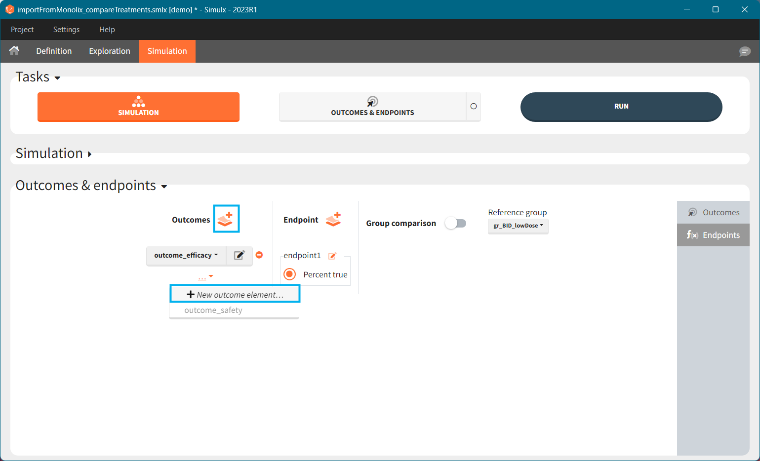
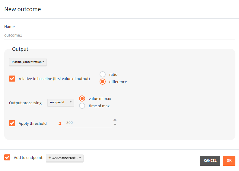
Each outcome has a name (default or user defined), which allows to select it in an endpoint definition. To define an outcome you have to select an output element for post – processing. You can only use output elements selected in the Simulation scenario. The specification of the outcome includes the following options to post-process the selected output.
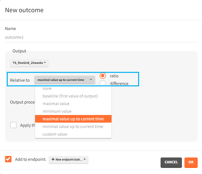
For continuous, count and categorical outputs:
Relative to: none/ baseline/ maximal or minimal value/ maximal or minimal value up to current time/ custom value: it divides (“ratio”) or subtracts (“difference”) the output values by the specific value (i.e baseline – the first value of the output). For baseline option, because the first value of the transformed output is non-informative (ratio=1 or difference=0), it is removed.
Output processing:
- average value – takes the average over all output values for each individual
- first or last value – takes a value at the first or last time point for each individual
- min or max value – takes the minimum or maximum over all output values for each individual. You can choose “value of min/max” to take the value of the min or max, or choose “time of min/max” to take the time of the min or max – as continues time or time-to-event.
- at custom point – takes a value of an output at a specified time point. Only grid time points are allowed.
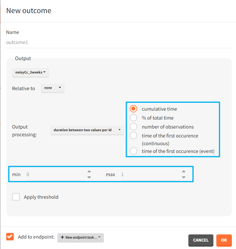
- duration below or above a value or between values – calculates time when the output values are below, above or between a given values. Strict inequalities (< or >) apply. You input threshold values manually below the output processing menu. As duration you can choose:
- “cumulative time” – sum of time intervals between consecutive time points where output values satisfy the condition
- “% of total time” – cumulative time divided by the final time (in percentage)
- “number of observations” – number of time points where output values satisfy the condition
- “time of the first occurrence” – a time point where the condition is satisfied for the first time (can be event or continuous)
Apply threshold: applies a logical test (usually comparing the outcome value to a threshold) to get a binary true/false outcome. You must set a threshold value and a comparison sign (=, !=, >=, <=, >, <).
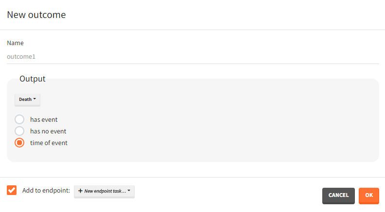
For single time-to-event outputs:
- Has event / has no event / time of event: “has event” and “has no event” calculates if the individual had or didn’t have an event during the observation period. This is a binary true/false outcome. “time of event” uses the TTE output as outcome directly. The outcome is then of type ‘time-to-event’.
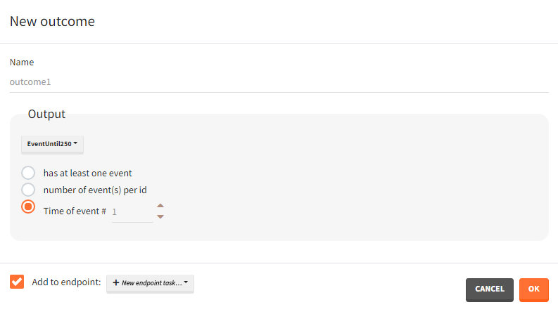
For repeated time-to-event outputs:
- Has at least one event / number of events per id / time of event #: “has at least one event” leads to a binary true/false outcome depending if the individual has at least one event during the observation period or not. “number of events per id” count the total number of events for each individual. This is an outcome of type ‘value’. “Time of event # “ generates a time-to-event outcome with a single event per individual. The index of the event to be considered can be typed-in by the user.
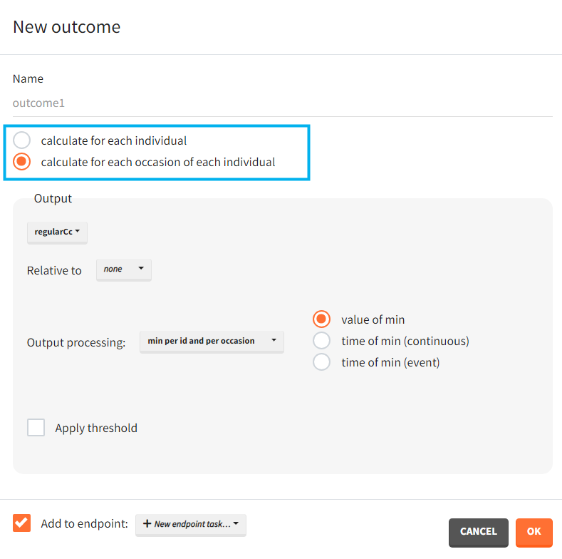
Occasions
In case occasions, you can choose to compute the outcome for each individual, or for each occasion of each individual. Select a corresponding radio button in the outcome definition window
Outcomes organization
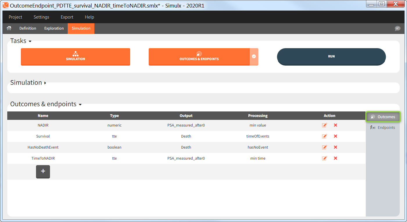
Outcomes are building blocks for endpoints. When you create a new outcome, you can add the outcome to a new or to an existing endpoint via the option “Add to endpoint” at the bottom of the outcome definition window. The Outcomes & endpoints section displays only the outcomes used in endpoints. All defined outcomes, whether used or not in an endpoint, appear in the list of outcomes:
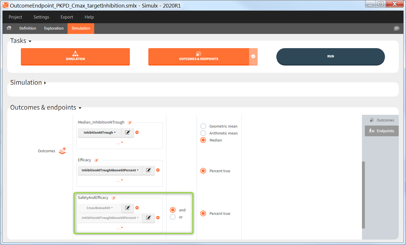
Outcomes of the same type can be combined together using AND/OR for binary true/false outcomes (e.g Cmax < threshold1 and Ctrough > threshold2), or MIN/MAX for double values and time-to-event (e.g max(CmaxParent, CmaxMetabolite) ).
Endpoints
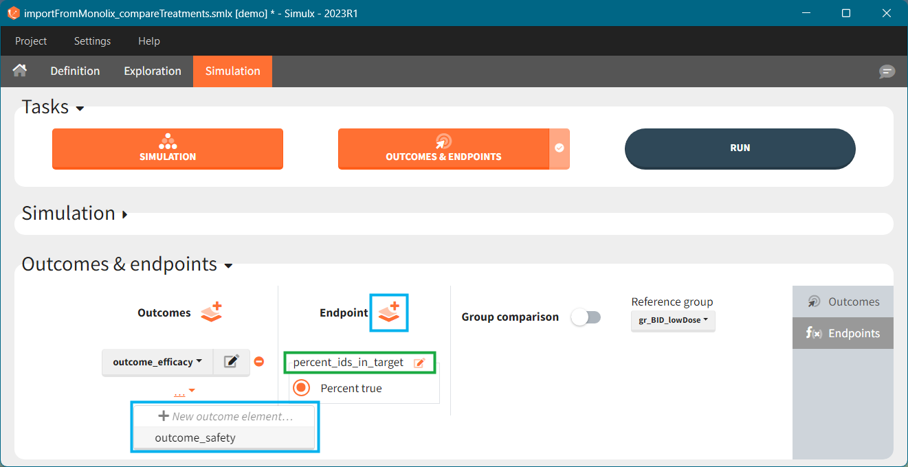
Endpoints summarize the outcome values over all individuals, for each simulation group and each replicate. To create a new endpoint, you can select one or several outcomes of the same type from the drop-down menu (highlighted below in blue) or click on the “+” icon next to the Endpoint header. Endpoints are also created automatically, when at the bottom of an outcome definition you select the option “Add to endpoint: New endpoint”. Once you create an endpoint, you can change its name highlighted below in green).
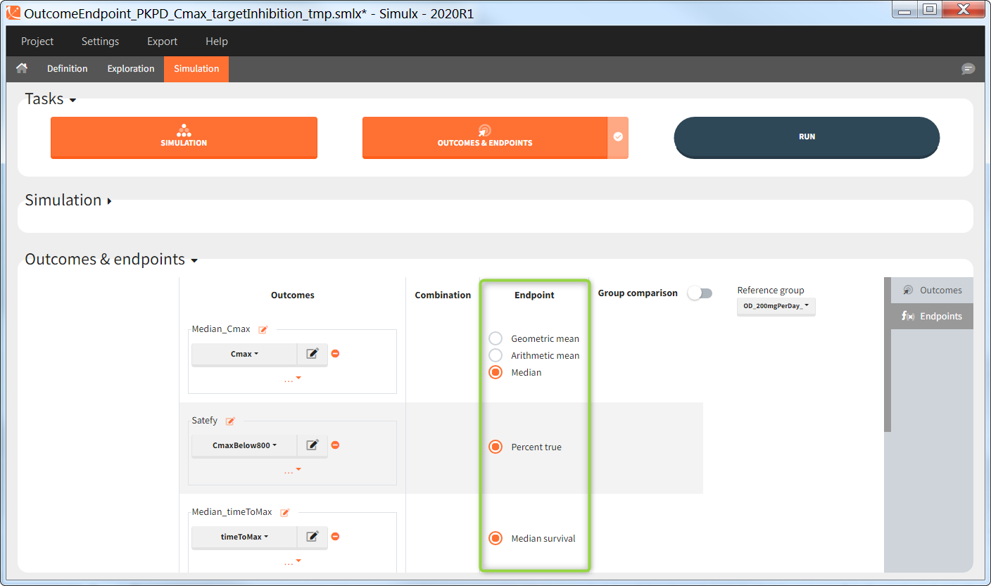
There are several options to summarize the individual outcomes into an endpoint. It depends on the type of outcomes:
- value outcomes: the endpoint can be
- geometric mean. Includes calculation of the coefficient of variation.
- arithmetic mean. Includes calculation of the standard deviation.
- median. Includes calculation of the 5th and 95th percentiles.
- binary true/false outcomes: the endpoint will be the percentage of true. Includes calculation of the “total number true”.
- time-to-event outcomes: the endpoint will be the median survival (time at which the Kaplan Meier curve is equal to 0.5). Includes calculation of the lower bound (5th) and and upper bound (95th) of the confidence interval of the median survival.
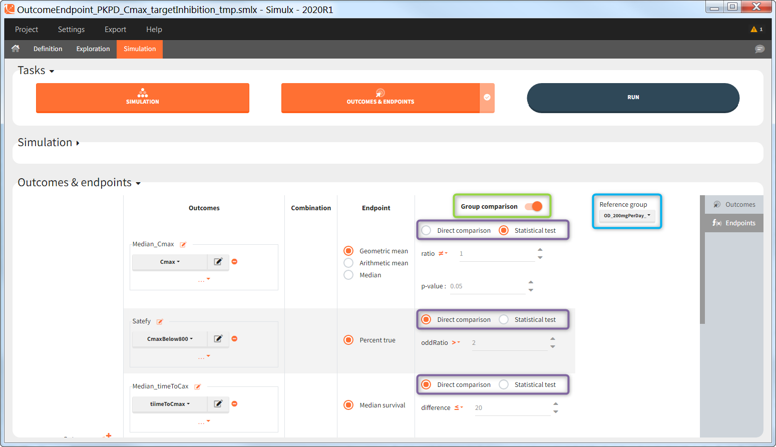
Group comparison
You can compare endpoints across simulation groups by activating the toggle “Group comparison” (green highlight). One of the simulation groups must be defined as the reference group (blue highlight) and all other groups will be compared to this reference group. For each endpoint, the group comparison can rely on a direct comparison of the endpoint values, or on a statistical test (purple highlight). The exact comparison or test applied depends on the type of the endpoint.
Statistical tests
This table gives an overview of the statistical tests performed in Group comparison depending on the type of outcome and endpoint. Next sections contain detailed information of each option.
| Outcome | Endpoint | Metric | Statistical test | |
| Same indiv = True | Same indiv = False | |||
| Continuous | Geometric mean | Ratio of means | Paired t-test on log-transformed |
Unpaired t-test on log-transformed |
| Arithmetic mean | Difference of means | Paired t-test | Unpaired t-test | |
| Median | Difference of medians | Wilcoxon signed rank test | Wilcoxon rank sum test | |
| Binary true/false | Percent true | Odds ratio | McNemar’s exact test | Fisher’s exact test |
| Time-to-event | Median survival | Difference in median survival | Logrank test with variance correction | Logrank test |
Endpoint “median” for value outcome
This test calculates the difference between the median of the test group and of the reference group: \( \textrm{median}_{test} – \textrm{median}_{ref} \) with \(\textrm{median}_{test}\) and \(\textrm{median}_{ref}\) the median in the test and reference group respectively.
In case of a direct comparison, this difference is compared using operators =, !=, >, >=, <, <= to a user-defined value (default: 0). When this logical comparison is true, the trial simulation is considered as ‘success’.
Example: When the direct comparison “difference > 25” is true, it means that the median in the test group is larger than in the reference group by at least 25 units (e.g ng/mL if the outcome is a peak concentration).
In case of a statistical test, a Wilcoxon rank sum test (equivalent to the Mann-Whitney test) (“Same individuals among groups” not selected) or a Wilcoxon signed rank test (“Same individuals among groups” selected) is done to compare the median of the test and reference group. “difference \(\neq\) 0” represents the alternative hypothesis H1. By default, it performs a two-sided test (sign \(\neq\)) and checks if the medians significantly differ from each other. You can define single-sided tests by choosing “>” or “<“. The minimal or maximal (depending of the direction of the test) difference can also be specified (default: 0). The statistical test results into a p-value, which is compared to a user-defined threshold (default: 0.05). If the p-value is below the threshold, the trial simulation is considered as ‘success’.
Example: When the statistical test testing the alternative H1 hypothesis “difference > 25” results into a small p-value, it means that the medians of the test and reference groups differ by more than 25 units significantly (e.g ng/mL if the outcome is a peak concentration) with a larger value for test.
Endpoint “arithmetic mean” for value outcome
This test calculates the difference between the mean of the test group and of the reference group: \( \textrm{mean}_{test} – \textrm{mean}_{ref} \) with \(\textrm{mean}_{test}\) and \(\textrm{mean}_{ref}\) the mean in the test and reference group respectively.
In case of a direct comparison, this difference is compared using operators =, !=, >, >=, <, <= to a user-defined value (default: 0). When this logical comparison is true, the trial simulation is considered as ‘success’.
Example: When the direct comparison “difference > 14 ” is true, it means that the mean in the test group is larger than in the reference group by at least 14 units (e.g ng/mL if the outcome is a peak concentration).
In case of a statistical test, it performs an unpaired t-test (“Same individuals among groups” not selected) or a paired t-test (“Same individuals among groups” selected) to compare the test and reference group. “difference \(\neq\) 0” represents the alternative hypothesis H1. By default, it performs a two-sided test (sign \(\neq\)) and checks if the two means significantly differ from each other. You can define single-sided tests by choosing “>” or “<“. The minimal or maximal (depending of the direction of the test) difference can also be specified (default: 0). The statistical test results into a p-value, and compares it to a user-defined threshold (default: 0.05). If the p-value is below the threshold, the trial simulation is considered as ‘success’.
Example: When the statistical test testing the alternative H1 hypothesis “difference > 14” results into a small p-value, it means that the means of the test and reference groups differ significantly by more than 14 units (e.g ng/mL if the outcome is a peak concentration) with a larger value for test.
Endpoint “geometric mean” for value outcome
This test calculates the ratio of the test geometric mean divided by the reference geometric mean: \( \textrm{geoMean}_{test} / \textrm{geoMean}_{ref} \) with \(\textrm{geoMean}_{test}\) and \(\textrm{geoMean}_{ref}\) the geometric mean in the test and reference group respectively.
In case of a direct comparison, this ratio is compared using operators =, !=, >, >=, <, <= to a user-defined value (default: 1). When this logical comparison is true, the trial simulation is considered as ‘success’.
Example: When the direct comparison “ratio > 2” is true, it means that the geometric mean in the test group is at least twice larger than in the reference group.
In case of a statistical test, it performs an unpaired t-test (“Same individuals among groups” not selected) or a paired t-test (“Same individuals among groups” selected) on the log-transformed values (which are assumed to follow a normal distribution) to compare the means of the test and reference group. “ratio \(\neq\) 1” represents the alternative hypothesis H1. By default, it performs a two-sided test (sign \(\neq\)) and checks if the geometric means significantly differ from each other. You can define single-sided tests by choosing “>” or “<“. The minimal or maximal (depending of the direction of the test) ratio can also be specified (default: 1). The statistical test results into a p-value, which is compared to a user-defined threshold (default: 0.05). If the p-value is below the threshold, the trial simulation is considered as ‘success’.
Example: When the statistical test testing the alternative H1 hypothesis “ratio > 2” results into a small p-value, it means that the geometric mean of the test group is significantly larger than twice the geometric mean of the reference group.
Endpoint “percent true” for binary true/false outcome
This test calculates the odds ratio between the test group and the reference group. The odds ratio definition is different depending if you use paired samples case or not.
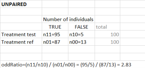
“Same individuals among groups” not selected (unpaired samples)
The odd ratio is \( \frac{pTest}{1-pTest} / \frac{pRef}{1-pRef} \) with \(pTest\) and \(pRef\) the fraction of true outcomes in the test and reference group respectively. \(1-pTest\) represents the fraction of false outcomes.
Equivalently, you can use the following contingency table to define the odd ratio.
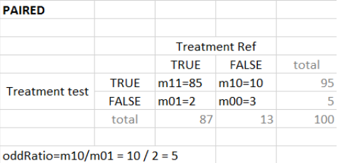
“Same individuals among groups” selected (paired samples)
In case of identical individuals among groups, the individuals which have the same outcome value in both groups (so Ref=True and Test=True, or Ref=False and Test=False) are not counted. The odd ratio is defined as\( \frac{nTest_TRef_F}{nTest_FRef_T}\), with \(nTest_TRef_F\) the number of individuals with true in the test group and and false in the reference group. It corresponds to the contingency table below. The odds ratio can frequently be zero or infinity – in particular in the absence of measurement noise – an individual true in the reference group is also necessarily true in the test group (corresponding for instance to a higher dose).
In case of a direct comparison, this odds ratio is compared using operators =, !=, >, >=, <, <= to a user-defined value (default: 1). When this logical comparison is true, the trial simulation is considered as ‘success’.
Example: When the direct comparison “odds ratio > 2” is true, it means that the odds in the test group are at least twice larger than in the reference group.
In case of a statistical test, it preforms a Fisher’s exact test (“Same individuals among groups” not selected) or a McNemar’s exact test (“Same individuals among groups” selected) to compare the results of the test and reference group via the construction of a 2×2 contingency table (which contain more information than the endpoinds \(pTest\) and \(pRef\)). “odds ratio \(\neq\) 1” represents the alternative hypothesis H1. By default, it performs a two-sided test (sign \(\neq\)) and checks if the odds ratio significantly differs from 1. You can define a single-sided tests by choosing “>” or “<“. The minimal or maximal (depending of the direction of the test) odds ratio can also be specified (default: 1). The statistical test results into a p-value, and compare it to a user-defined threshold (default: 0.05). If the p-value is below the threshold, the trial simulation is considered as ‘success’.
Example: When the statistical test testing the alternative H1 hypothesis “odds ratio > 2” results into a small p-value, it means that the odds of the test group are significantly larger than twice the odds of the reference group.
Endpoint “median survival” for time-to-event outcome
This test calculates the difference between the median survival of the test group and of the reference group: \( \textrm{medSurv}_{test} – \textrm{medSurv}_{ref} \) with \(\textrm{medSurv}_{test}\) and \(\textrm{medSurv}_{ref}\) the median survival (time at which the Kaplan-Meier estimates equals 0.5) in the test and reference group respectively.
In case of a direct comparison, this difference is compared using operators =, !=, >, >=, <, <= to a user-defined value (default: 1). When this logical comparison is true, the trial simulation is considered as ‘success’.
Example: Direct comparison “difference > 60” corresponds to median survival in the test group larger than in the reference group by 60 time units (e.g days).
In case of a statistical test, it performs a logrank test to compare the survival Kaplan-Meier curves. Selecting “Same individuals among groups”, applies a variance correction (see Jung 1999). “difference \(\neq\) 0” represents the alternative hypothesis H1. By default, it performs a two-sided test (sign \(\neq\)) and checks if the survival curves significantly differ. You can define single-sided tests by choosing “>” or “<“. For the log rank test, it is not possible to define a “minimal difference”. The statistical test gives a p-value, and compare it to a user-defined threshold (default: 0.05). If the p-value is below the threshold, the trial simulation is considered as ‘success’.
Example: When the statistical test testing the alternative H1 hypothesis “difference \(\neq\) 0” results into a small p-value, it means that the survival curves from the two groups differ significantly.
