RsSimulx simulx() function

simulx(): simulation of mixed effects models and longitudinal data

Description

Compute predictions and sample data from Mlxtran and R models

Usage

simulx(
  model = NULL,
  parameter = NULL,
  covariate = NULL,
  output = NULL,
  treatment = NULL,
  regressor = NULL,
  occasion = NULL,
  varlevel = NULL,
  group = NULL,
  project = NULL,
  nrep = 1,
  npop = NULL,
  fim = NULL,
  saveSmlxProject = NULL,
  result.file = NULL,
  addlines = NULL,
  settings = NULL
)

Arguments

`model`	(string) a Mlxtran model used for the simulation. It can be a text file or an output of the inLine function.
`parameter`	One of a vector of parameters with their names and values, a dataframe with parameters defined for each id or each pop a string, path to a data frame (csv or txt file) a string corresponding to the parameter elements automatically generated by monolix (only when simulation is based on a Monolix project). One of the following mlx parameter elements: “mlx_Pop”, “mlx_PopUncertainSA”, “mlx_PopUncertainLin”, “mlx_PopIndiv”, “mlx_PopIndivCov”,”mlx_CondMean”, “mlx_EBEs”,”mlx_CondDistSample”
`covariate`	One of a vector of covariates with their names and values. a dataframe with covariates defined for each id a string, path to a data frame (csv or txt file) a string corresponding to the covariate elements automatically generated by monolix (only when simulation is based on a Monolix project). One of the following mlx covariate elements: “mlx_Cov” and “mlx_CovDist”
`output`	output or list of outputs. An output can be defined by a string corresponding to the output elements automatically generated by monolix (only when simulation is based on a Monolix project) – the format is mlx_nameofoutput. a list with fields `name`: a vector of output names `time`: a vector of times a dataframe with columns id, time (columns lloq, uloq, limit are optional) a string, path to a data frame (csv or txt file) `lloq`: lower limit of quantification (when time is a vector of times) `uloq`: upper limit of quantification (when time is a vector of times) `limit`: lower bound of the censoring interval (when time is a vector of times)
`treatment`	treatment or list of treatments. A treatment can be defined by A list with fields `time`: a vector of input times, `amount`: a scalar or a vector of amounts, `rate`: a scalar or a vector of infusion rates (default=Inf), `tinf`: a scalar or a vector of infusion times (default=0), `washout`: a scalar or a vector of boolean (default=F), `adm`: (or type) the administration type (default=1), `repeats`: the treatment cycle (optional), a vector with fields `cycleDuration`: the duration of a cycle, `NumberOfRepetitions`: the number of cycle repetition `probaMissDose`: the probability to miss each dose (optional). a dataframe with treatments defined for each id a string, path to a data frame (csv or txt file) a string corresponding to the treatment elements automatically generated by monolix (only when simulation is based on a Monolix project) – for example mlx_Adm1.
`regressor`	treatment or list of treatments. A treatment can be defined by a list with fields `name`: a vector of regressor names, `time`: a vector of times, `value`: a vector of values. a dataframe with columns id, time, and regressor values a string, path to a data frame (csv or txt file)
`occasion`	An occasion can be defined by A list with fields `name`: name of the variable which defines the occasions, `time`: a vector of times (beginnings of occasions) A dataframe with columns id, time, occasion a string, path to a data frame (csv or txt file) “none”, to delete an occasion structure
`varlevel`	deprecated, use occasion instead.
`group`	a list, or a list of lists, with fields: `size`: size of the group (default=1), `parameter`: if different parameters per group are defined, `covariate`: if different covariates per group are defined, `output`: if different outputs per group are defined, `treatment`: if different treatments per group are defined, `regressor`: if different regression variables per group are defined. “level” field is not supported anymore in RsSimulx.
`project`	the name of a Monolix project
`nrep`	Samples with or without uncertainty depending which element is given as “parameter”.
`npop`	deprecated, set parameter = “mlx_popUncertainSA” or “mlx_popUncertainLin” instead.
`fim`	deprecated, set parameter = “mlx_popUncertainSA” or “mlx_popUncertainLin” instead.
`saveSmlxProject`	If specified, smlx project will be save in th path location (by default smlx project is not saved)
`result.file`	deprecated
`addlines`	a list with fields: `formula`: string, or vector of strings, to be inserted . “section”, “block” field are not supported anymore in RsSimulx. You only need to specify a formula. The additional lines will be added in a new section EQUATION.
`settings`	a list of optional settings `seed`: initialization of the random number generator (integer) (by default a random seed will be generated) `id.out`: add (TRUE) / remove (FALSE) columns id and group when only one element (N = 1 or group = 1) (default=FALSE) `kw.max`: deprecated. `replacement`: deprecated, use samplingMethod instead `samplingMethod`: str, Sampling method used for the simulation. One of “keepOrder”, “withReplacement”, “withoutReplacement” (default “keepOrder”) `out.trt`: TRUE/FALSE (default = TRUE) output of simulx includes treatment `sharedIds`: Vector of Elements that share ids. Available types are “covariate”, “output”, “treatment”, “regressor”, “population”, “individual” (default c()) `sameIndividualsAmongGroups`: boolean, if True same individuals will be simulated among all groups (default False) `exportData`: boolean, if True and if a path to save the smlx project (saveSmlxProject) is specified, export the simulated dataset (smlx project directory/Simulation/simulatedData.txt) (default False)

Details

simulx takes advantage of the modularity of hierarchical models for simulating different components of a model: models for population parameters, individual covariates, individual parameters and longitudinal data.

Furthermore, simulx allows to draw different types of longitudinal data, including continuous, count, categorical, and time-to-event data.

The models are encoded using either the model coding language Mlxtran. Mlxtran models are automatically converted into C++ codes, compiled on the fly and linked to R using the RJSONIO package. That allows one to implement very easily complex models and to take advantage of the numerical sovers used by the C++ mlxLibrary.

Value

A list of data frames. Each data frame is an output of Simulx

Examples

Example 1: simulation from scratch

This example shows how to create a Simulation from scratch and plot the results.

myModel <- inlineModel("
  [LONGITUDINAL]
  input = {A, k, c, a}
  EQUATION:
  t0 = 0
  f_0 = A
  ddt_f = -k*f/(c+f)
  DEFINITION:
  y = {distribution=normal, prediction=f, sd=a}
  [INDIVIDUAL]
  input = {k_pop, omega}
  DEFINITION:
  k = {distribution=lognormal, prediction=k_pop, sd=omega}
")

f <- list(name='f', time=seq(0, 30, by=0.1))
y <- list(name='y', time=seq(0, 30, by=2))
parameter <- c(A=100, k_pop=6, omega=0.3, c=10, a=2)

res <- simulx(model = myModel,
parameter = parameter,
occasion = data.frame(time=c(0, 0), occ=c(1, 2)),
output = list(f,y),
group = list(size=4),
saveSmlxProject = "./project.smlx")

res <- simulx(model = myModel,
parameter = parameter,
occasion = data.frame(time = c(0, 0, 0, 0),
occ1 = c(1, 1, 2, 2),
occ2 = c(1, 2, 3, 4)),
output = list(f,y),
group = list(size=4))

res <- simulx(model = myModel,
parameter = parameter,
output = list(f,y),
group = list(size=4))

plot(ggplotmlx() + geom_line(data=res$f, aes(x=time, y=f, colour=id)) +
geom_point(data=res$y, aes(x=time, y=y, colour=id)))
print(res$parameter)

Example 2: simulation from a Monolix project

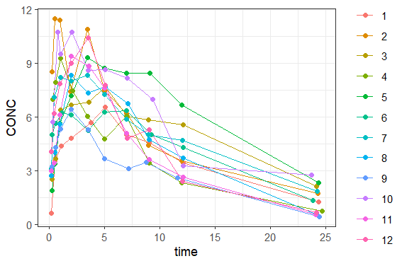
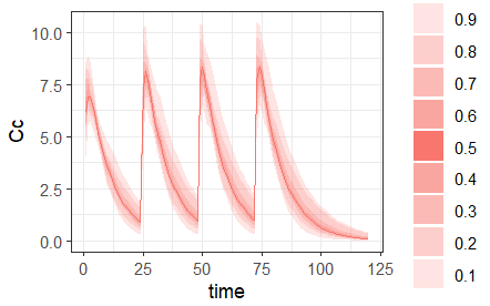
This example shows how to simulate from a Monolix project (using a Monolix demo): first with all the simulation elements exported from Monolix (Simulx resimulates the dataset from Monolix using the population parameter estimated in the Monolix project), then with a new design for the treatment (4 doses are given to all individuals), output (Cc is recorded instead of CONC, so the residual error is not included in the simulations) and group size (20 simulated individuals).

# First use the Monolix connectors to get the path to the demos and estimate the population parameters of the Monolix project
library(lixoftConnectors)
initializeLixoftConnectors(software = "monolix")
demoProject <- paste0(getDemoPath(),"/1.creating_and_using_models/1.1.libraries_of_models/theophylline_project.mlxtran")
loadProject(demoProject)
runPopulationParameterEstimation()

# Then use RsSimulx for the simulations
library(RsSimulx)

res <- simulx(project = demoProject)
plot(ggplotmlx() + geom_line(data=res$CONC, aes(x=time, y=CONC, colour=id)) +
geom_point(data=res$CONC, aes(x=time, y=CONC, colour=id)))

res <- simulx(project = demoProject, 
              treatment = list(time=seq(0, by=24,length=4), amount=4), 
              group = list(size=20), 
              output = list(name="Cc", time=1:120)) 

prctilemlx(res$Cc)