
1.Overview
Version 2024
This documentation is for Simulx.
©Lixoft
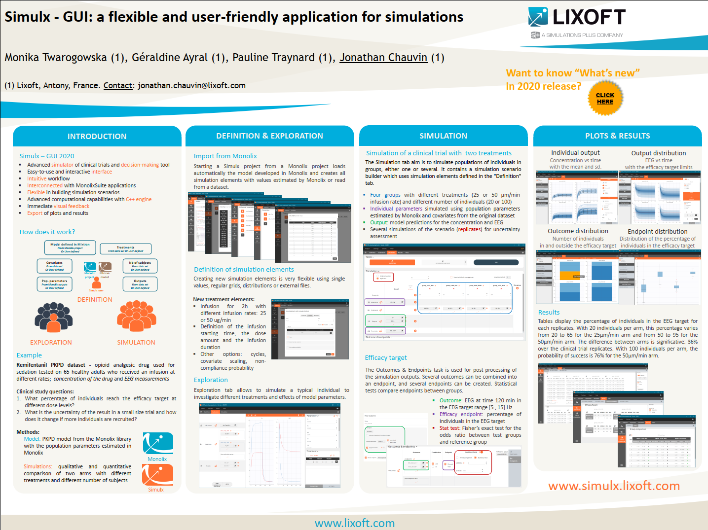
Simulx GUI – easy, efficient and flexible application for clinical trial simulations
Now, more than ever, to increase drug success rate and accelerate clinical development it is important to incorporate new technology – like clinical trials simulators. They improve the quality and efficiency of decision making process. Modeling&simulation approach models molecules and mechanisms from the available data and then uses these models to generate new information that can optimize your strategies in terms of time, money and commercial success.
What if it were possible to:
- Use your estimated model and, investigating new dosing regimens and populations, gain unique insights that improve your chances of success?
- Avoid costly surprises by simulating easily different scenarios with a flexible and user-friendly interface?
- Utilize the outputs from simulations to optimize your clinical trial strategies that reduces drug development cycle?
It is possible to do this, and more, with Simulx GUI!
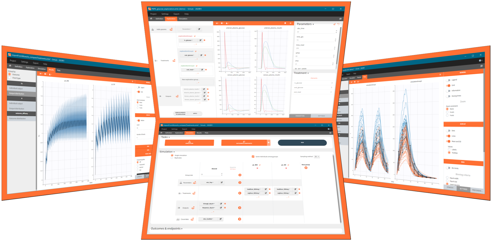
Simulx is an advanced simulation software interconnected with Monolix and flexible in building user-designed scenarios. This application combines a user-friendly interface with the highest computational capabilities to help you make faster and more informed decisions.
Simulx has three sections that create an optimal environment to build and analyse simulations:
-
- Definition – create easily new exploration and simulation elements of different types.
- Exploration – explore different treatments and effects of model parameters on a typical individual.
- Simulation – simulate a clinical trial using a population of individuals in one or several groups with specific treatment or features and use flexible post-processing tools, clear results and interactive plots for analysis.
How does it work?
Start with:
play:
- add new dosing regimens, parameters, covariates, outputs, etc.
- explore effects of model parameters and treatments
- combine defined elements into a desired simulation with one or several groups for comparison
- create outcomes&endpoints to quantify the simulations outputs
- start immediately the analysis and decision process using automatically generated results and plots
and customize:
- plots: add analysis features, stratify data and modify plotting area look
- interface: use dark theme and increase font size and numbers precision
- data: save user files in the result folder
- export: data, plots and settings
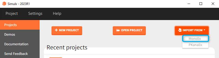
1.1.Import a project from Monolix
There are three methods to start a project in Simulx: create a new project, open an existing project and import a project from Monolix or PKanalix. To import a project from Monolix is as simple as clicking on the button “Import from Monolix” in the Simulx home tab. It is the easiest way to build a simulation scenario, because everything to run a simulation is prepared automatically. As a result, it saves a lot of time.You can always modify current simulation elements, define new ones and change the scenario, so the flexibility of Simulx is not compromised.
1. Simulx project structure with “Import from Monolix”
2. A typical simulation workflow with a project imported from Monolix
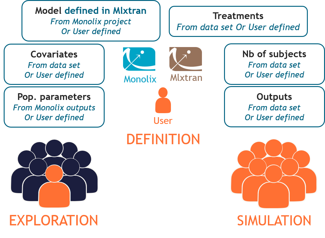
Simulx project structure
Importing a project from Monolix creates a Simulx project with pre-defined elements. You can use them to re-simulate the dataset from the Monolix project or as a base for a new simulation scenario. These elements appear in the Definition tab:
- Model, population parameters and individual parameters estimates and output variables are imported from Monolix.
- Occasions, covariates, treatments and regressors are imported from the dataset (used in the imported Monolix project).
Simulx sets default exploration and simulation scenarios – they are ready to run. They contain one exploration group to simulate a typical individual (in the exploration tab) and one simulation group to re-simulate the Monolix project (in the simulation tab).
Default simulation elements
- model: mlxtran model with blocks [INDIVIDUAL], [COVARIATE] and [LONGITUDINAL].
- pop.params.:
- mlx_PopInit [no POP.PARAM task results]: (vector) initial values of the population parameters from Monolix.
- mlx_Pop: (vector) population parameters estimated by Monolix.
- mlx_PopUncertainSA (resp. mlx_PopUncertainLin): (matrix) an element which enables to sample population parameters using the covariance matrix of the estimates computed by Monolix if the Standard Error task (Estimation of the Fisher Information matrix) was performed by stochastic approximation (resp. by linearization). To sample several population parameter sets, this element needs to be used with replicates.
- indiv.params.:
- mlx_IndivInit [no POP.PARAM task results]: (vector) initial values of the population parameters from Monolix.
- mlx_PopIndiv: (vector) population parameters estimated by Monolix.
- mlx_PopIndivCov: (table) population parameters with the impact of the covariates used in the model (but no random effects).
- mlx_EBEs: (table) EBEs (conditional mode) estimated by Monolix.
- mlx_CondMean: (table) conditional mean estimated by Monolix.
- mlx_CondDistSample: (table) one sample of the conditional distribution (first replicate in Monolix).
- covariates [if used in the model]:
- mlx_Cov: (table) ids and covariates read from the dataset.
- mlx_CovDist: (distribution) distribution of covariates from the dataset with empirical mean and variance for continuous covariates, set as lognormal for positive continuous covariates, normal for continuous covariate with some negative values, and multinomial low based on frequencies of modalities for categorical covariates.
- treatment:
- mlx_AdmID: (table) ids, amounts and dosing times (+ tinf/rate or washouts) read from the dataset for each administration type.
- outputs:
- mlx_observationName: (table) ids and measurement times read from the dataset for each output of the observation model
- mlx_predictionName: (vector) uniform time grid with 250 points on the same time interval as the observations for each continuous output of the structural model.
- mlx_TableName: (vector) uniform time grid with 250 points on the same time interval as the observations for each variable of the structural model defined as table in the OUTPUT block.
- occasions:
- mlx_Occ [if used in the model]: (table) ids, times and occ(s) read from the dataset.
- regressors:
- mlx_Reg [if used in the model]: (table) ids, times and regressor values and names read from the dataset.
Default exploration and simulation scenarios
Exploration:
- Indiv.params: mlx_IndivInit or mlx_PopIndiv.
- Treatment: one exploration group with mlx_AdmId for all administration IDs.
- Output: mlx_predictionName for all predictions defined in the model.
Simulation:
- Size: number of individuals read from the dataset.
- Parameters: mlx_PopInit or mlx_Pop.
- Treatment: mlx_AdmId for all administration IDs.
- Output: mlx_observationName for all observations.
- Covariates: mlx_cov if used in the model.
- Regressor: mlx_reg if used in the model.
Interface allows to have an overview on all defined elements, modify them and create new ones as well as build simulation scenarios. But, if you modify the imported model, then Simulx will remove all simulation elements. In addition, if you remove occasions, then all occasion-dependent simulation elements will be removed as well.
A typical simulation workflow with a project imported from Monolix
The projects shown here are available as demo projects in the interface “1.overview – importFromMonolix_xxx.smlx”:
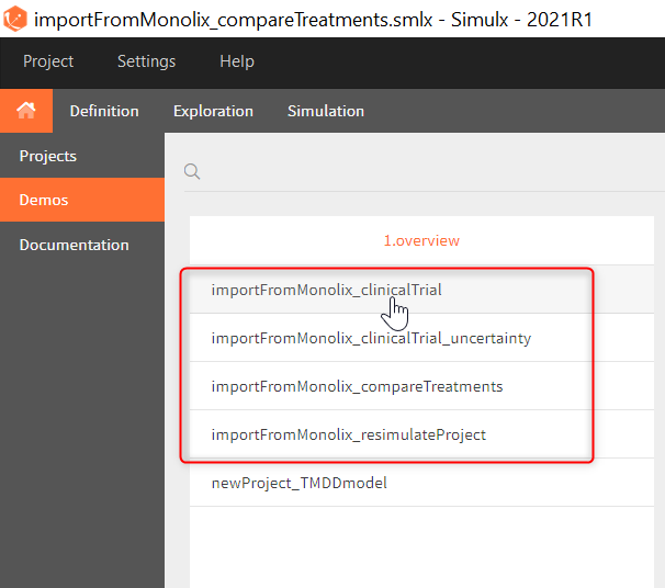
This example is based on a PK-PD model for Warfarin developed and estimated in Monolix. The Warfarin dataset contains concentration and PCA(%) measurements for 32 individuals, who received different oral doses of the drug. Firstly, the goal of the Simulx project is to use the information from the Monolix project to test the efficacy and safety conditions for different treatments. Secondly, to simulate clinical trials and compare various dosing regimens strategies. Simulations should answer the following questions:
- Which “loading dose” strategy assures a rapid steady state without a concentration peak?
- Do multi-dose treatments meet the efficacy and safety criteria?
- What is the uncertainty of the percentage of individuals in a target due to the variability between individuals and due to the size of a trial group?
Model:
The PK model includes an administration with a first order absorption and a lag time. It has one compartment and a linear elimination. The PD model is an indirect turnover model with inhibition of the production. All individual parameters have log-normal distribution besides the Imax parameter, which is logitNormally distributed. In addition, the log-transformed scaled weight covariate explains intra-individual variability of the volume, age covariate has an effect on the clearance and sex covariate on the baseline response. Finally, the combined-1 error model is used in the observation model of the concentration, and the constant model of the response.
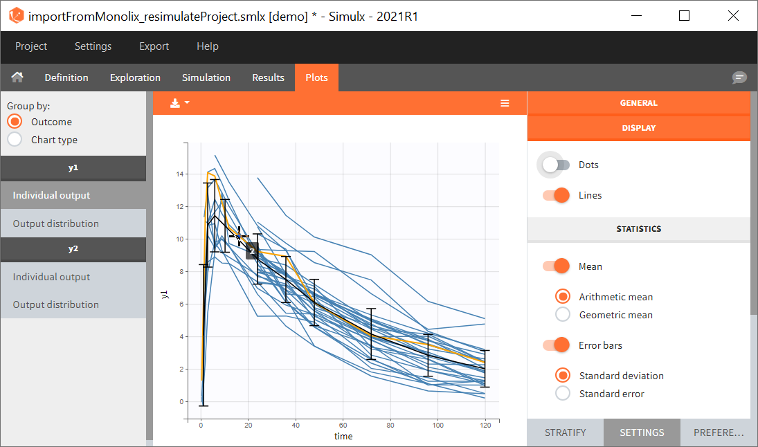
0. Re-simulation of the Monolix project
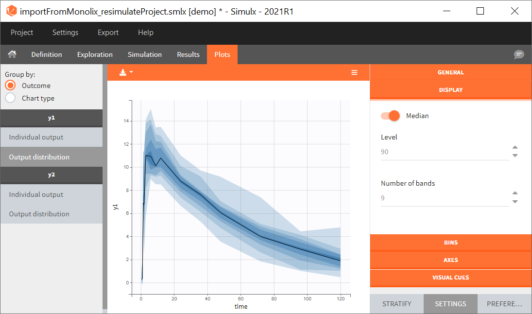
[Demo project “1.overview – importFromMonolix_resimulateProject.smlx”]
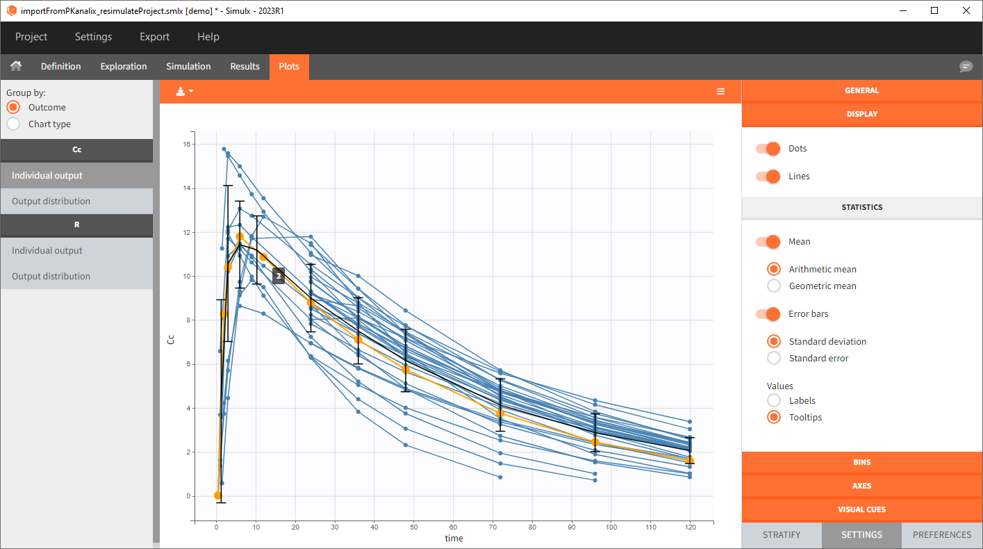
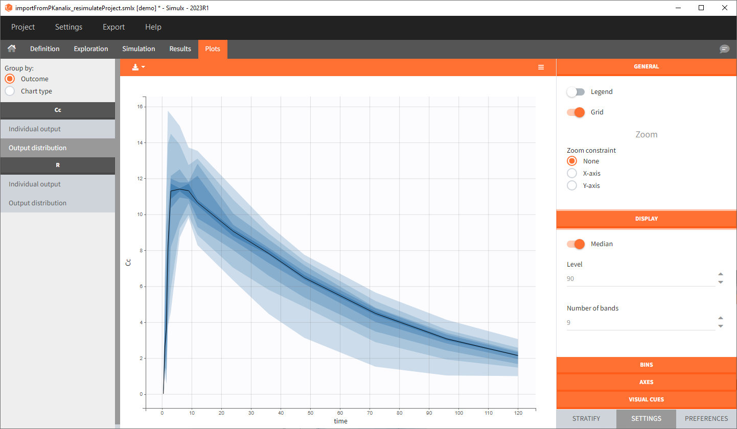
You can download the Monolix project for this example, here. To import it in SImulx, first unzip the folder, then start a Simulx session, click on “Import from: Monolix” and browse the .mlxtran file. After importing a project from Monolix, the task buttons “simulation” and “run” in the Simulation tab re-simulate the project. Plots and results are generated automatically. Results are tables for outputs and individual parameters and plots display model observations as individual outputs and distributions.
1. Exploration of the loading dose strategies
[Demo project “1.overview – importFromMonolix_compareTreatments.smlx”]
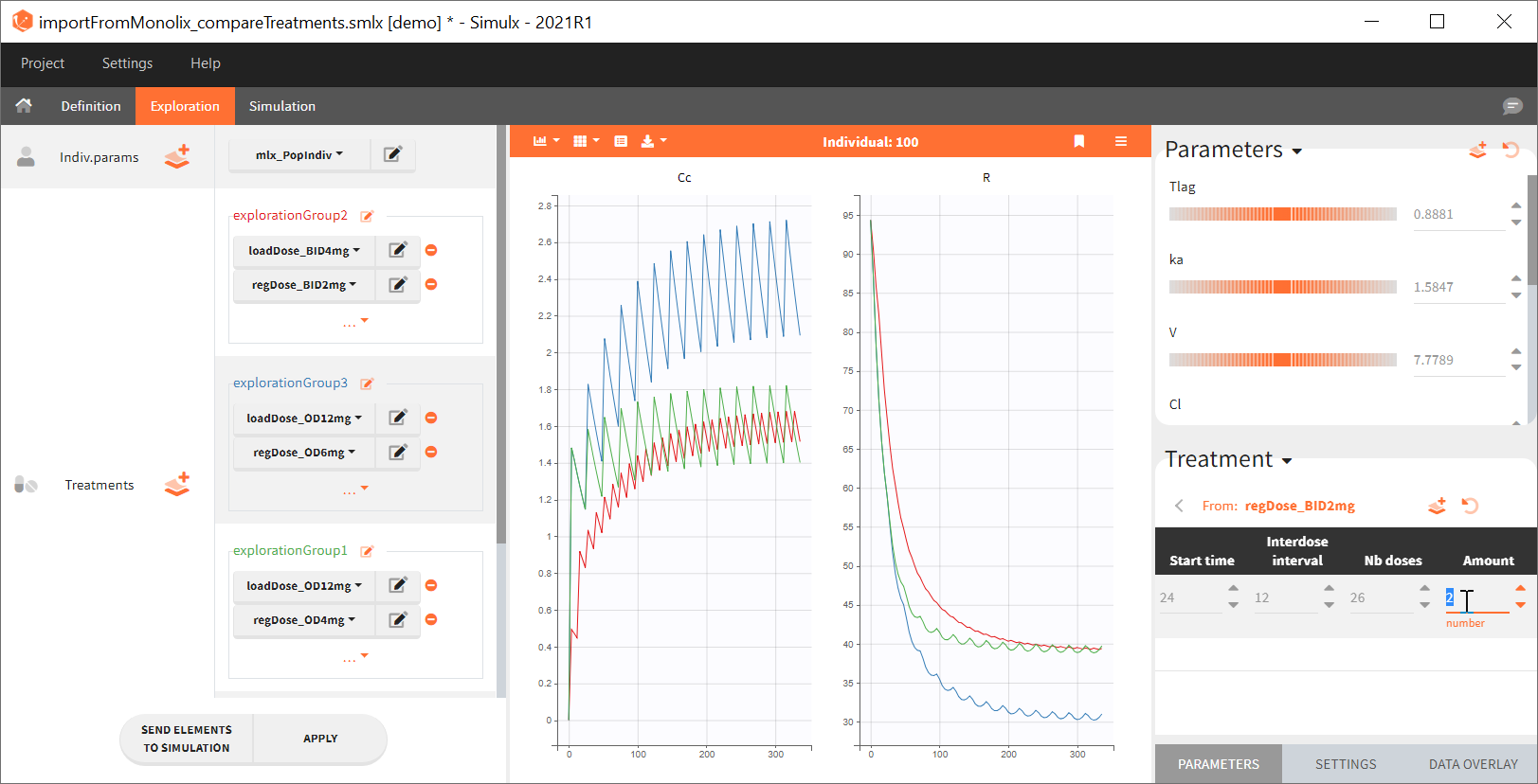
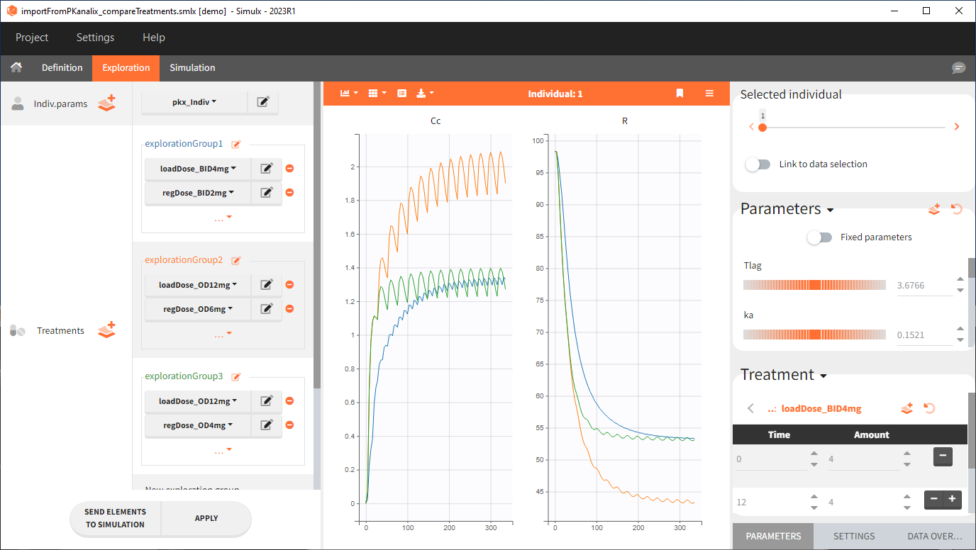
Exploration tab simulates a typical individual. After importing a project from Monolix (the same as in the previous example), you can choose different types of individual parameters elements, eg. equal to population parameters estimated by Monolix or EBEs. Using several exploration groups allows to compare different treatments in one chart. The goal of this example is to test how many days of a “loading dose” are necessary to reach a steady state without a peak of the concentration. Starting dosing regimens are:
- 1 day with a load dose 12mg OD followed by 13 days with a 6mg single dose OD
- 1 day with a load dose 12mg OD followed by 13 days with a 4mg single dose OD
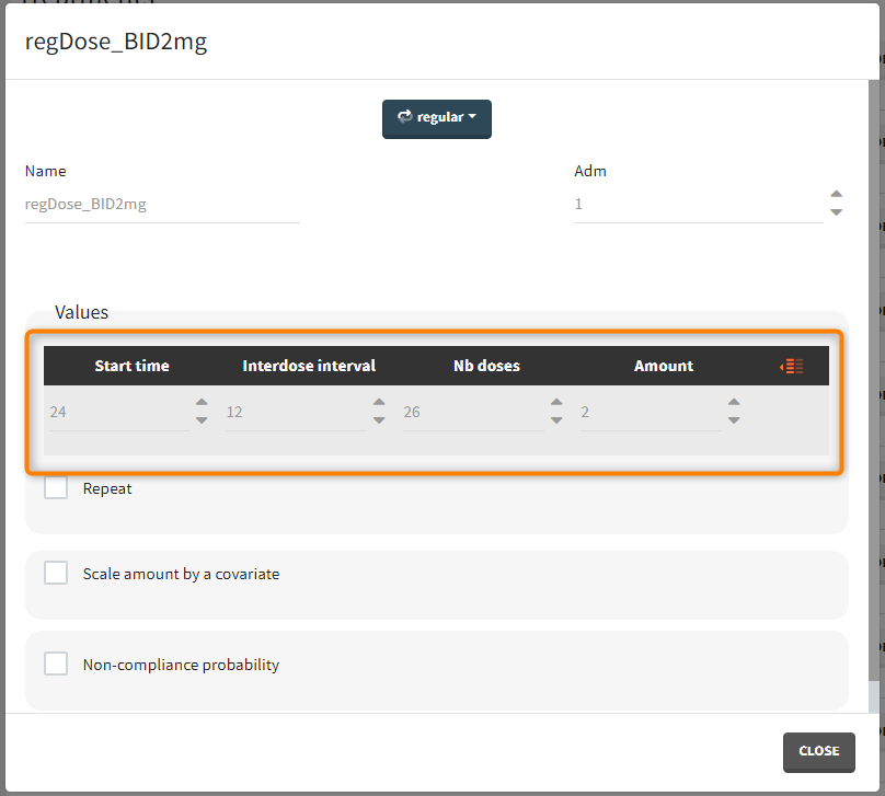
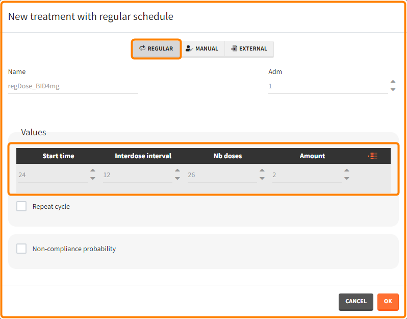
- 1 day with load doses 4mg twice a day (BID) followed by 26 doses of 2mg every 12 hours.
“Loading dose” treatments elements are of manual type (with time of a dose and amount), while multi-dose elements are of regular type. Regular type includes a specification of a treatment period, inter-dose interval and number of doses. You combine treatments elements directly in the exploration tab (in the left panel).
Output is the concentration prediction Cc and the response prediction R on a regular time grid over the whole treatment period (t = 0:1:336) . The plot displays one subplot per output, and all exploration groups (=dosing regimen) together on each subplot. In the right panel, you can edit treatment elements and parameters interactively – predictions are updated on-the-fly for all groups to help you find which exact regimen is the most promising.
2. Treatment comparison: percentage of individuals in the target
[Demo project “1.overview – importFromMonolix_compareTreatments.smlx”]
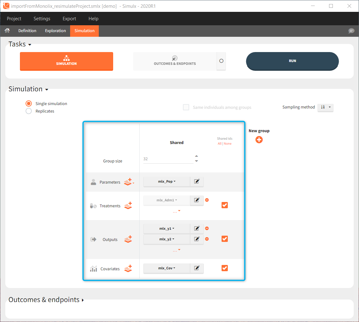
Simulation scenario
Exploration tab performed simulation on one individual. In the simulation tab, Simulx simulates a population of individuals. SImulation outputs can be further post-processed to calculate, for example, the percentage of individuals in the target for different treatment arms. This simulation scenario uses the following treatment and output elements.
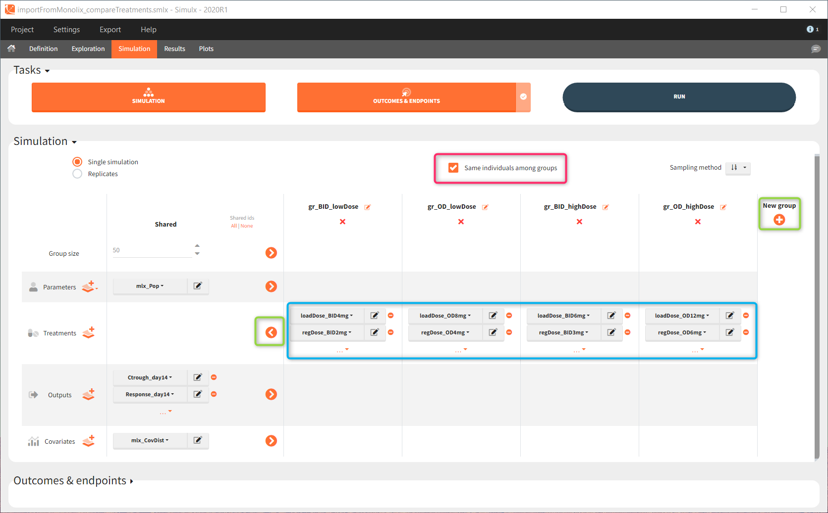
- BID treatment: One day of a “loading dose” with 4mg or 6mg dose twice a day (BID), followed by 26 doses of 2mg or 3 mg respectively each 12 hours.
- OD treatment: One day of a “loading dose” with 8mg or 12mg dose once a day (OD), followed by 13 doses of 4mg or 6 mg respectively each 24 hours.
- Outputs: manual type using model predictions (Cc and R) at time equal 336h.
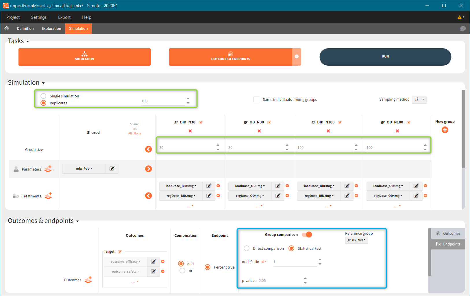
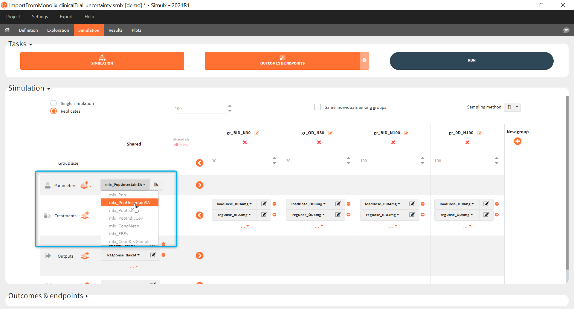
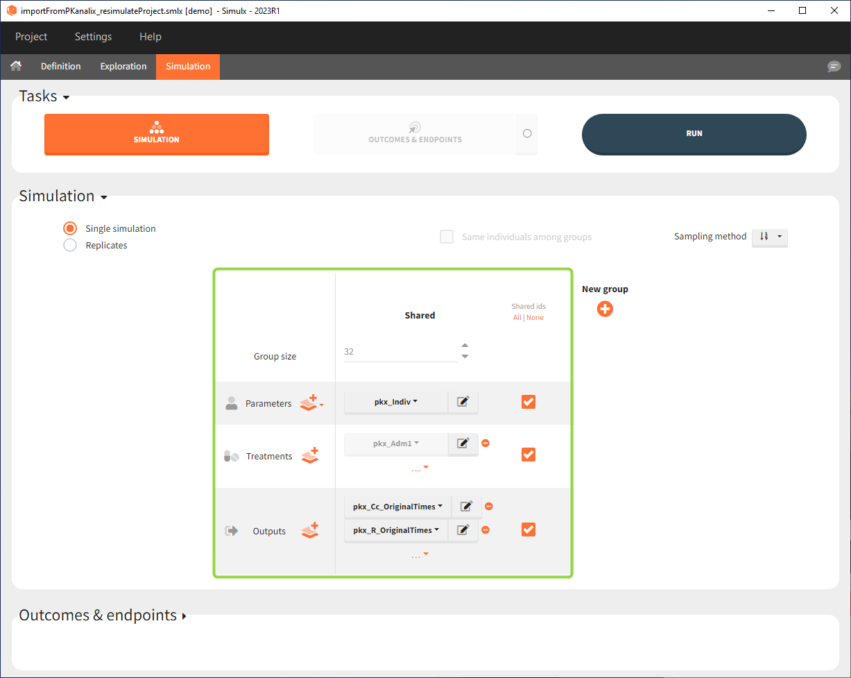
In the simulation tab, the button “plus” adds a new group and “arrows” (green frames below) move elements from the shared section to the group specific section. For treatment, each group has a specific combination of treatments (blue frame). In addition, the option “same individuals among groups” removes the effect of intra-individual variability between individuals (red frame). As a consequence, the observed differences between groups are only due to the treatment and simulation can use a smaller number of individuals.
The comparison between groups is in terms of the percentage of individuals in the efficacy and safety target:
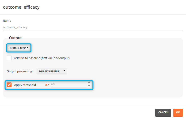
- Efficacy: PCA at the end of the treatment should be less than 60%.
- Safety: Ctrough on the last treatment day should be less than 2ug/mL.
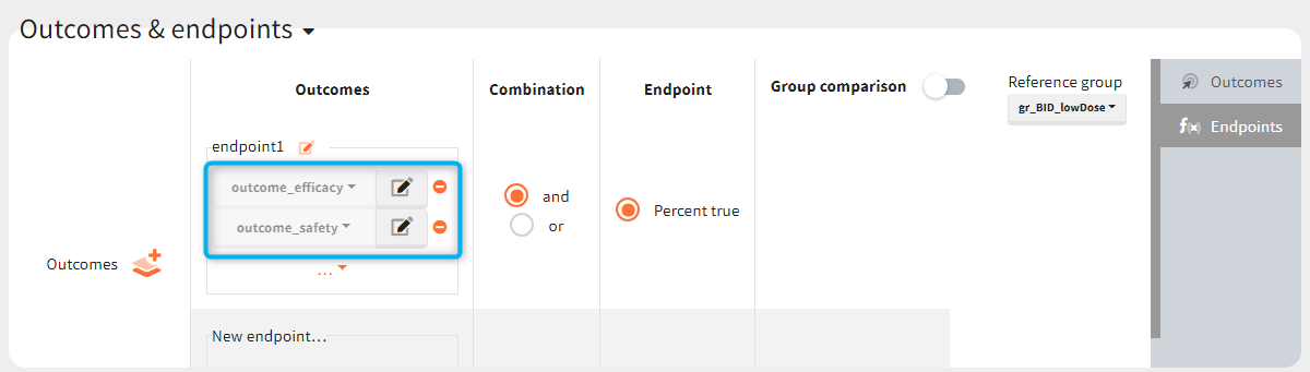
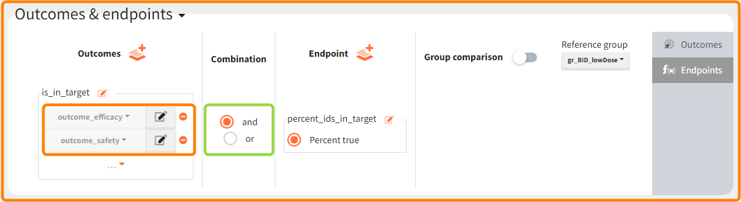
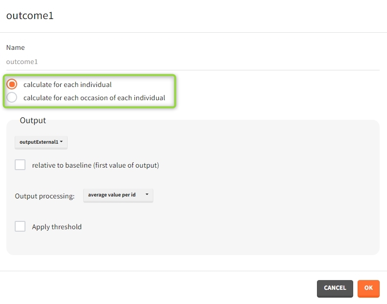
You can calculate it in the outcomes&endpoints section of the simulation tab. Definition of new outcomes includes selecting an output computed in the simulation scenario and post-processing methods. When you apply threshold condition, then outcome is of a binary (true/false) type.
In addition, outcomes can be combined together (blue frame below), and an endpoint summarizes “true” outcomes over all individuals in groups.
Analysis
Similarly to the task button “Simulation”, which runs the simulation, the “Outcomes & endpoint” button performs post-processing, which in this example means calculating the efficacy and safety criteria and the number of individuals in the target. When you run this task, SImulx generates automatically the results in the “endpoint” section and plots for outcomes distributions.
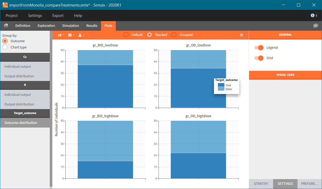
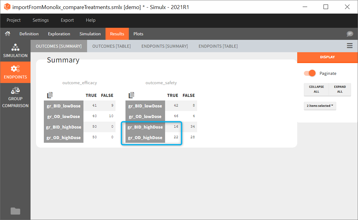
In this example, the outcome distribution compares the number of individuals in the target between groups. The highest number of “true” outcomes is in the group with the low level dose twice a day (gr_BID_lowDose). Failure to satisfy the safety criteria by the two groups with the high dose level causes large numbers of “false” outcomes. In fact, the endpoint results show that for these two groups less than half of the individuals have Ctrough below the safety threshold (blue frame below).
3. Clinical trial simulation and uncertainty of the results
[Demo project “1.overview – importFromMonolix_clinicalTrial.smlx”]
The previous step shows that the high dose level violates the safety criteria in more than 50% of individuals. Therefore, the simulation of a clinical trial uses only one dose level with the BID and OD administration.
The goal is to analyse the effect of the uncertainty due to the variability between individuals, measurement errors and number of individuals in a trial.
New simulation scenario has four groups which combine different dosing regimens (BID or OD) with different group sizes (30 or 100). Outputs are model observations at the end of the treatment. To simulates the scenario several times (green frames), use the option “replicates”. As a result, the endpoints summarize the outcomes not only over the groups but also over the replicates.
[Starting from the demo project “1.overview – compareTreatments.smlx”, change number of replicates to 100, and add two groups: one with treatment as for GR_BID, other as GR_OD. Move “number of ids” as group specific, and set N=30 for one BID-OD pair and N=100 for the other. Change names to indicate group sizes.]
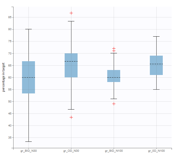
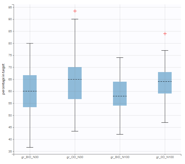
After running both tasks, plots display the endpoint distribution as a box plot with the mean value (dashed line) and standard deviations for each group. As expected, the uncertainty is lower for trial with more individuals. However, the mean values remain at similar levels.
“Group comparison” option in the Outcomes&endpoints section compares the endpoints values across groups (blue frame). Selecting different reference groups and hypothesis (through the odds ratio) allows to change the objectives. Moreover, calculation of new outcomes or endpoints do not require re-running a simulation because the post-processing is a separate task.
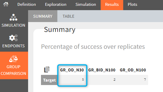
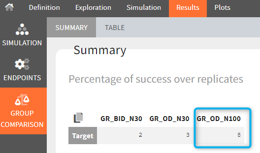
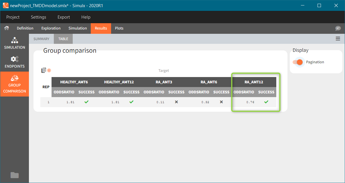
The statistical test checks if any of the dosing regimens, BID or OD, is better than the other. Firstly, in the smaller trial so the gr_BID_N30 group is the reference and the hypothesis states that the odds ratio is different from one. For each replicate, if the p-value is lower than selected 0.05, then a test group (GR_OD_N30) is a “success”. Results summary in the “group comparison” section shows that only 5% of the test group replicates are successful (upper image below), which suggests that OD dosing regimen is not significantly better than BID. Larger trial size might give different results. Change reference group to gr_BID_N100 and re-run the outcomes & endpoints task. Percentage of successful replicates for gr_OD_N100 is higher, 8%, (lower image below), but it is comparable to the previous result.
4. Propagation of parameter uncertainty to the predictions
[Demo project in 2021 version only “1.overview – importFromMonolix_clinicalTrial_uncertainty.smlx”]
In the previous step, we replicated the study 100 times to check the impact of sampling different individuals on the endpoint, and on the power of the study. For all these replicates, we sampled individuals using the same population parameters (so same typical values and deviations of random effects).
The goal of this final step is to check the impact of the uncertainty of population parameter estimates on the final endpoint and study power. For this, starting from the 2021 version, it is possible to use the population parameter element mlx_PopUncertainSA (resp. mlx_PopUncertainLin) if standard errors have been computed by stochastic approximation in the original Monolix project (resp. by linearization). Now the 100 replicates will be samples using each time different population parameter values, which are sampled from the variance-covariance matrix of the estimates imported from Monolix.
When running again simulation and outcomes with this population parameter element, we obtain a higher uncertainty on the endpoint than in step 3, since now we observe in addition the uncertainty related to the estimation of parameters in Monolix.
1.2.Import a project from PKanalix
There are three methods to start a project in Simulx: create a new project, open an existing project and from Monolix to Simulx or import project from PKanalix. To import a project from PKanalix, simply click the “Import from PKanalix” option of the “Import from” in the Simulx Home tab. It is the most convenient way to create a simulation scenario, as everything is automatically prepared for running a simulation.You can modify current simulation elements, define new ones and change the scenario at any time, such that the flexibility of Simulx is not compromised.
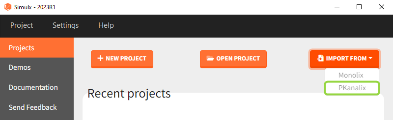
1. Simulx project structure with “Import from PKanalix”
2. A typical simulation workflow with a project imported from PKanalix
Simulx project structure
Importing a project from PKanalix creates a Simulx project with pre-defined elements. You can use them to re-simulate the dataset from the PKanalix project or as a base for a new simulation scenario. These elements appear in the Definition tab:
- Model, individual parameters estimates and output variables are imported from PKanalix.
- Occasions, treatments and regressors are imported from the dataset.
Moreover, exploration and simulation scenarios are set and ready to run. They contain one exploration group to simulate a typical individual (in the exploration tab) and one simulation group to re-simulate the PKanalix project (in the simulation tab).
Default simulation elements
- model: same structural model as in the CA Model tab of PKanalix. Model is written in mlxtran language
- Indiv.params.:
- pkx_IndivInit [no POP.PARAM task results]: (vector) individual parameters corresponding to the initial values of the parameters in PKanalix
- pkx_Indiv: (table) individual parameters estimated by CA task
- pkx_IndivGeoMean: (vector) geometric mean of individual parameters over all subjects
-
- pkx_AdmID: (table) ids, amounts and dosing times (+ tinf/rate or washouts) read from the dataset for each administration type.
- outputs:
- pkx_ outputName_ FineGrid (vector): for each continuous output of the structural model, a vector with a uniform time grid with 250 points on the same time interval as the observations.
- pkx_ outputName_OriginalTimes (table): for each output of the model, a table with values for ids and observation times corresponding to the measurements read from the dataset
- pkx_TableName: (vector) for each variable of the structural model defined as table in the OUTPUT block, a vector with a uniform time grid with 250 points on the same time interval as the observations.
- occasions:
- pkx_Occ [if used in the model]: (table) ids, times and occ(s) read from the dataset.
- regressors:
- pkx_Reg [if used in the model]: (table) ids, times and regressor values and names read from the dataset.
Default exploration and simulation scenarios
Exploration:
- Indiv.params: pkx_Indiv or pkx_IndivInit.
- Treatment: one exploration group with pkx_AdmId for all administration IDs.
- Output: pkx_outputName_FineGrid for all predictions defined in the model on a fine time grid.
Simulation:
- Size: number of individuals read from the dataset.
- Parameters: pkx_Indiv or pkx_IndivInit.
- Treatment: mlx_AdmId for all administration IDs.
- Output: pkx_outputName_OriginalTimes for all model outputs.
- Regressor: pkx_reg if used in the model.
 Interface allows to have an overview on all defined elements, modify them and create new ones as well as build simulation scenarios. But, if you modify the imported model, then Simulx will remove all simulation elements. In addition, if you remove occasions, then all occasion-dependent simulation elements will be removed as well.
A typical simulation workflow with a project imported from PKanalix
The projects shown here are available as demo projects in the interface “1.overview – importFromPKanalix_xxx.smlx”: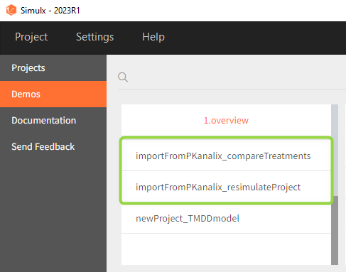
This example is based on a PK-PD model for Warfarin developed and estimated in Monolix. The Warfarin dataset contains concentration and PCA(%) measurements for 32 individuals, who received different oral doses of the drug with the amount 1.5mg/kg. Both the PKPD model and the PKPD parameter estimates come from the compartment analysis (CA) performed in PKanalix. The aim of the Simulx project is to to use the information from the PKanalix project to test the efficacy and safety conditions for different treatments. Possible questions to answer with simulations:
- Which “loading dose” strategy assures a rapid steady state without a concentration peak?
- Do multi-dose treatments meet the efficacy and safety criteria?
Model:
The PK model includes an administration with a first order absorption and a lag time. It has one compartment and a linear elimination. The PD model is an indirect turnover model with inhibition of the production.
0. Re-simulation of the PKanalix project
[Demo project “1.overview – importFromPKanalix_resimulateProject.smlx”]
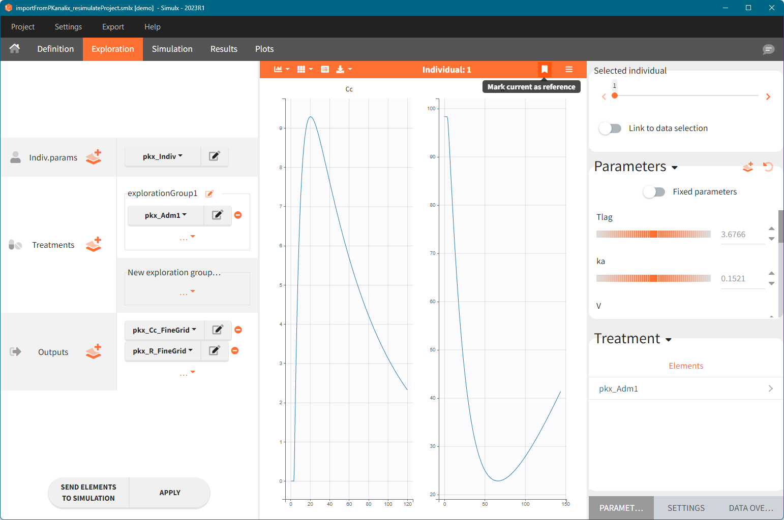
You can download the PKanalix project for this example, here. To import it in Simulx, first unzip the folder, then start a Simulx session, click on “Import from: PKanalix” and browse the .pkx file. After importing a project from PKanalix, the task buttons “simulation” and “run” in the Simulation tab re-simulate the project. Plots and results are generated automatically. Results are tables for outputs and individual parameters and plots display model observations as individual outputs and distributions.
1. Exploration of the loading dose strategies
[Demo project “1.overview – importFromPKanalix_compareTreatments.smlx”]
Definition
The Exploration tab simulates a typical individual. After importing a project (the same as in the previous example), you can choose different types of individual parameters elements, eg. individual parameters estimated in the CA task or geometric mean estimated over all individual parameters. Using several exploration groups allows to compare different treatments in one chart. The goal of this example is to test how many days of a “loading dose” are necessary to reach a steady state without a peak of the concentration. Starting dosing regimens are:
- 1 day with a load dose 12mg OD followed by 13 days with a 6mg single dose OD
- 1 day with a load dose 12mg OD followed by 13 days with a 4mg single dose OD
- 1 day with load doses 4mg twice a day (BID) followed by 26 doses of 2mg every 12 hours.
“Loading dose” treatments elements are of manual type (with time of a dose and amount), while multi-dose elements are of regular type. Regular type includes a specification of a treatment period, inter-dose interval and number of doses. You combine treatments elements directly in the exploration tab (in the left panel).
Exploration
Output is the concentration prediction Cc and the response prediction R on a regular time grid over the whole treatment period (t = 0:1:336) . The plot displays one subplot per output, and all exploration groups (=dosing regimen) together on each subplot. In the right panel, you can edit treatment elements and parameters interactively – predictions are updated on-the-fly for all groups to help you find which exact regimen is the most promising.
2. Treatment comparison: percentage of individuals in the target
[Demo project “1.overview – importFromPKanalix_compareTreatments.smlx”]
Simulation scenario
Exploration tab performed simulation on one individual. In the simulation tab, Simulx simulates a population of individuals – in this case all individuals from the original dataset used in the imported PKanalix project. Simulation outputs can be further post-processed to calculate, for example, the percentage of individuals in the target for different treatment arms. This simulation scenario uses the following treatment and output elements.
- BID treatment: One day of a “loading dose” with 4mg or 6mg dose twice a day (BID), followed by 26 doses of 2mg or 3 mg respectively each 12 hours.
- OD treatment: One day of a “loading dose” with 8mg or 12mg dose once a day (OD), followed by 13 doses of 4mg or 6 mg respectively each 24 hours.
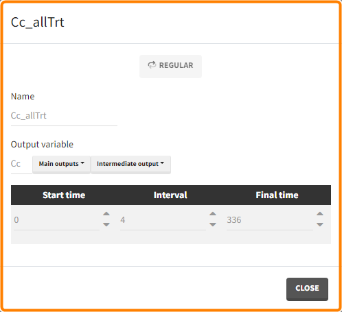
- Outputs: regular type using model predictions (Cc and R) up to time 336h.

The Simulation tab consists of the same element blocks as the Exploration tab. the button “plus” adds a new group and “arrows” (green frames below) move elements from the shared section to the group specific section. For treatment, each group has a specific combination of treatments (orange frame). As output a new vector was defined. Click on the “edit” icon to see the time discretization. Both output vectors, for the concentration as well as for the response range from time point 0 to time point 336 with step size 4 (unit is in hours h).
The option “Same individual among groups” removes the effect of intra-individual variability between individuals (red frame). As a consequence, the observed differences between groups are only due to the treatment itself. This case
Outcomes & endpoints
The efficacy and safety criteria correspond to the following conditions:
- Efficacy: at the end of the treatment PCA should not exceed 60%.
- Safety: on the last treatment day concentration should not exceed 1.5µg/mL
You can calculate it in the outcomes&endpoints section of the simulation tab. Definition of new outcomes includes selecting an output computed in the simulation scenario and post-processing methods. When you apply threshold condition, then outcome is of a binary (true/false) type.

In addition, the defined outcomes can be combined together with a logical operator (green frames below), and an endpoint summarizes “true” outcomes over all individuals in groups.
Analysis
Analogous to the “Simulation” button that runs the simulation, the ” Outcomes & Endpoint” button performs the post-processing – calculates the efficacy and safety criteria and the number of people in the target. In addition, the execution of this task automatically generates the results in the “Endpoint” section and graphs for the outcomes distributions.
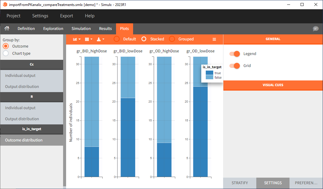
In this example, the outcome distribution compares the number of individuals in the target between treatment groups. Stack charts show the highest number of ” true ” results (\(\widehat{=}\) at time t=336h PCA \(\le\) 60% AND Cc \(\le\) 1.5µg/mL) in the group with the low dose once daily (gr_OD_lowDose).
Large number of “false” in the two groups with the high doses (gr_OD_highDose, gr_BID_highDose) relates to the violation of the safety criteria. The endpoint results show that for these two groups, less than 1/3 of the subjects have concentration below the safety threshold (green frame below).
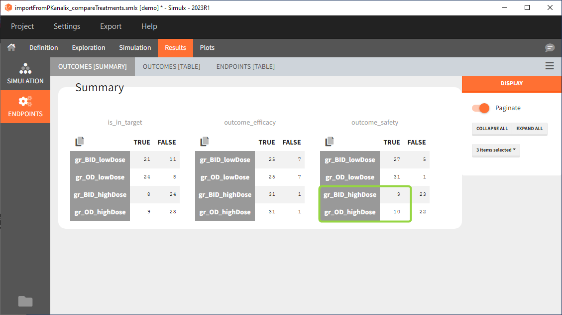
Conclusion
In the higher multi-dose regimens, although 31 of 32 subjects reach the efficacy criterion, only 9 to 10 of these subjects meet the safety criterion.
The group with the lower dose administered once per day, gr_OD_lowDose, have the highest success rate: 24 out of 32 subjects, i.e. 75% of the subjects meet both the safety and the efficacy criteria.
Go to typical simulation workflow with a project imported from Monolix, to see how you can extend this analysis to simulations of clinical trials and assessment of the uncertainty.
1.3.New project from scratch
New possibilities, as well as unexpected and unwanted effects, arise during different phases of drugs development. Simulx allows to create a new project from scratch, which gives freedom in simulating new scenarios. Moreover, it creates easily a space for testing new hypothesis. This helps to explore the full potential of drugs, and better prepare for their possible failures.
To create a new project from scratch:
- Select “New project” after opening the Simulx.
- Browse, or write new, mlxtran model (see here for details about the model structure).
- Use Definition tab to specify simulation elements required by the model. Explore in the Exploration tab the effects of treatments and parameters. Build a simulation scenario in the Simulation tab and run the simulation.
Demo project: 1.overview/newProject_TMDDmodel
The following example shows how to build “from scratch” a simulation that aims at comparing different treatments among two populations: healthy volunteers and patients with rheumatoid arthritis. It uses a TMDD model for a ligand and receptor concentrations. In addition, the synthesis of the receptor depends on the population type – lower for healthy subjects. All simulation elements are user-defined. The basic assumption is that a treatment is effective if the free receptor stays below 10% of the baseline. The goal is to test if the dose levels effective on healthy volunteers allow rheumatoid arthritis patients to reach the efficiency target.
Model
When building a project from scratch, loading a model is mandatory and has to be done in the first place. It sets automatically the structure of a simulation based on the model type and its elements.
- Structural model is a TMDD model with the QE approximation, two compartments and oral administration.
- Statistical model defines an effect of the patient state (healthy or with RA) on the synthesis rate of the receptor. It also includes the power law relationship between the weight covariate and the volume of the central compartment.
Covariates and their transformations are described in the [COVARIATE] block, the statistical model of the individual parameters is in the [INDIVIDUAL] block, while the [LONGITUDINAL] block contains the structural model with output definitions.
Definition of the scenario elements:
To guide building a project from scratch, Simulx defines default simulation elements automatically using information from the loaded model. These elements can be removed or modified, as well as new elements can be created. In this example, the definition includes the following new elements used in the exploration and simulation.
- Pop.Param.: Values come from an external table with at least two mandatory rows. The first row contains names of all population parameters as used in the model, while the second has the parameter values.
- Indiv.Params.: Individual parameters appear in the exploration tab. In this example, they are equal to population parameters in order to explore the effect of parameters on the model predictions for a typical individual.
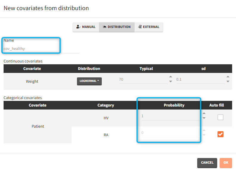
- Covariates: The aim of this simulation is to compare two populations (healthy and with rheumatoid arthritis). There are two covariate elements with different values of the “patient” covariate, but the same “weight” covariate.
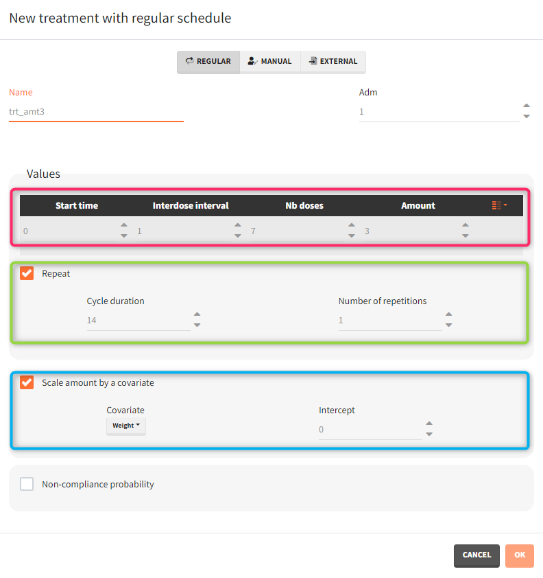
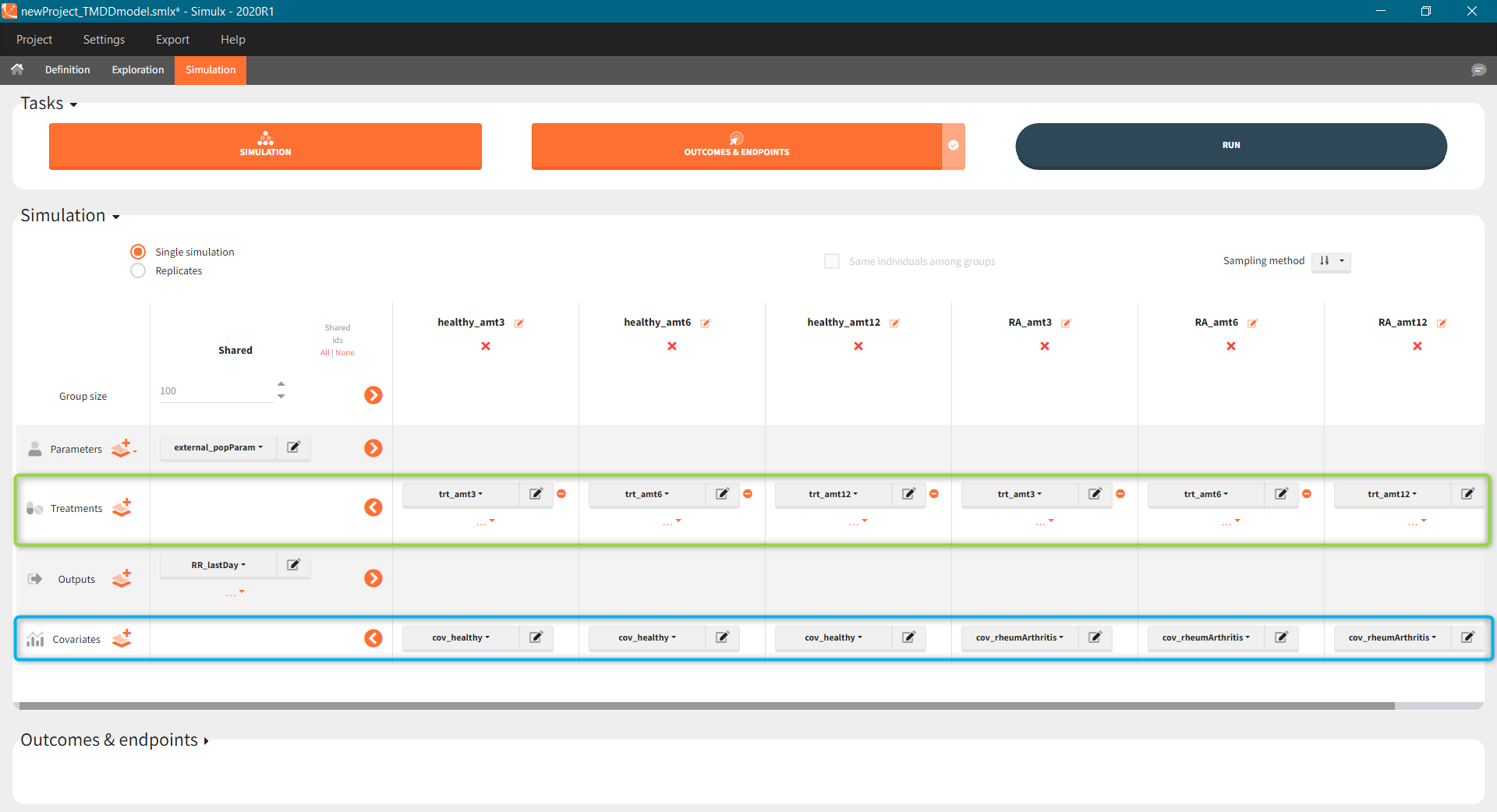
- Treatment has two cycles (green frame). In each cycle patients receive an oral dose scaled by their weight (blue frame) once per day for 7 days (red frame) followed by 7 days without a treatment. Three different dose levels: 3mg/kg, 6mg/kg and 12mg/kg require three separate treatment elements . An option “duplicate” allows to clone a treatment, and then change only the name and the amount. Note that the “View” option has the scaling formula.
- Outputs elements include the ratio between the free receptor and the baseline. This output on the regular grid is useful in the exploration. Simulation uses only the value at the end of the treatment. The latter choice speeds up the computations in case of many individuals and/or replicates.
Exploration
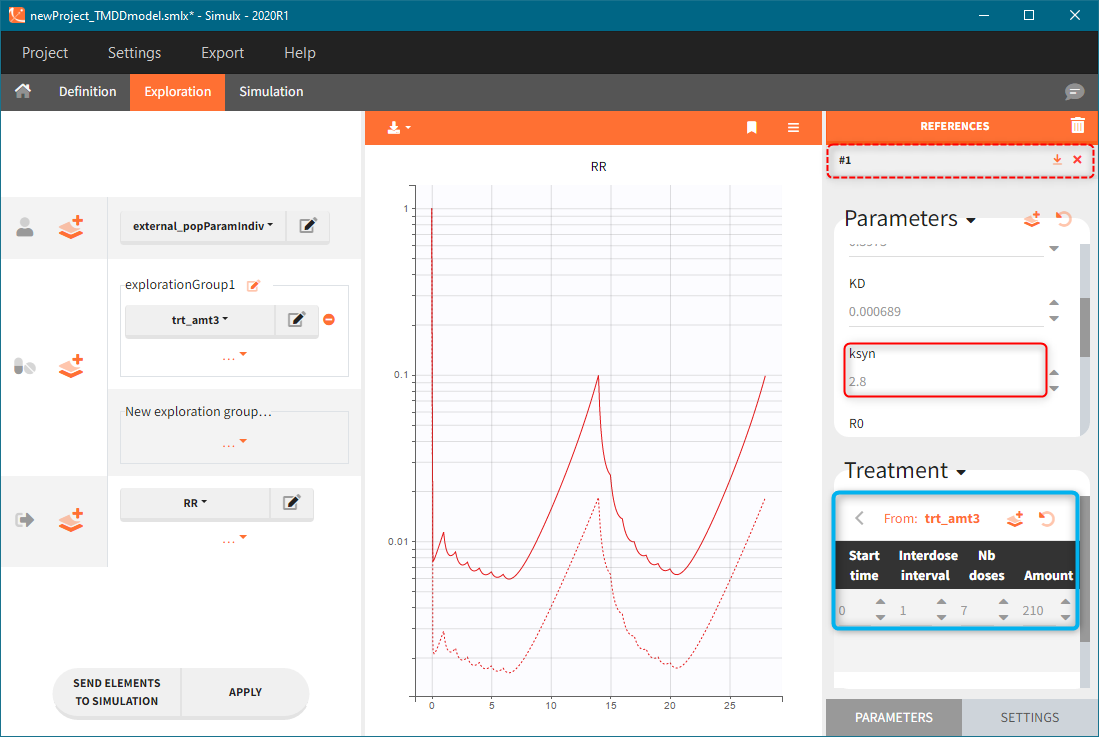
The model assumes that rheumatoid arthritis disease affects the synthesis of the free receptor (ksyn parameter). It means that for a certain dose level the efficacy target can be reached by healthy individuals (ksyn_pop = 0.789, dashed reference curve in the figure below), but not by patients with rheumatoid arthritis (ksyn_pop = 2.8, solid curve). In this exploration, the scaling of the amount 3mg/kg corresponds to typical individual with a weight 70kg (blue frame).
Simulation
The scenario consists of 6 groups for three dose levels and two populations, see here to learn about creating a simulation scenario.
- Treatment is group specific. Each group uses one of the three covariate dependent doses: 3mg/kg, 6mg/kg or 12mg/kg (green frame).
- Type of a population – healthy or with the rheumatoid arthritis – is in the group specific covariate (blue frame).
- Group size, population parameters and the output are the same for all groups.
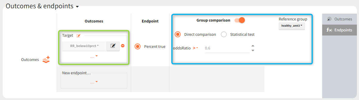
The outcomes&endpoints section defines post-processing of the simulation outputs for post-processing, which helps to compare the groups. The main endpoint is the percentage of individuals reaching the efficacy target in each group. It summarizes the “true” outcomes, which correspond to the situation when the ratio between the free receptor and the baseline at the end of the treatment is less then 10% (green frame). In addition, the “group comparison” (blue frame) compares the endpoints of all groups with respect to the reference group (healthy population with 3mg/kg dose level).
Results
To run the simulation and the calculation of the endpoints it is enough to select both tasks and click the button “Run”. Generation of the results and plots is automatic in two dedicated tabs. The outcome distribution shows that the efficacy of the treatment in healthy individuals stays above 90% (red line) for all dose levels. On the contrary, a group with rheumatoid arthritis achieves this level only at the highest tested dose.
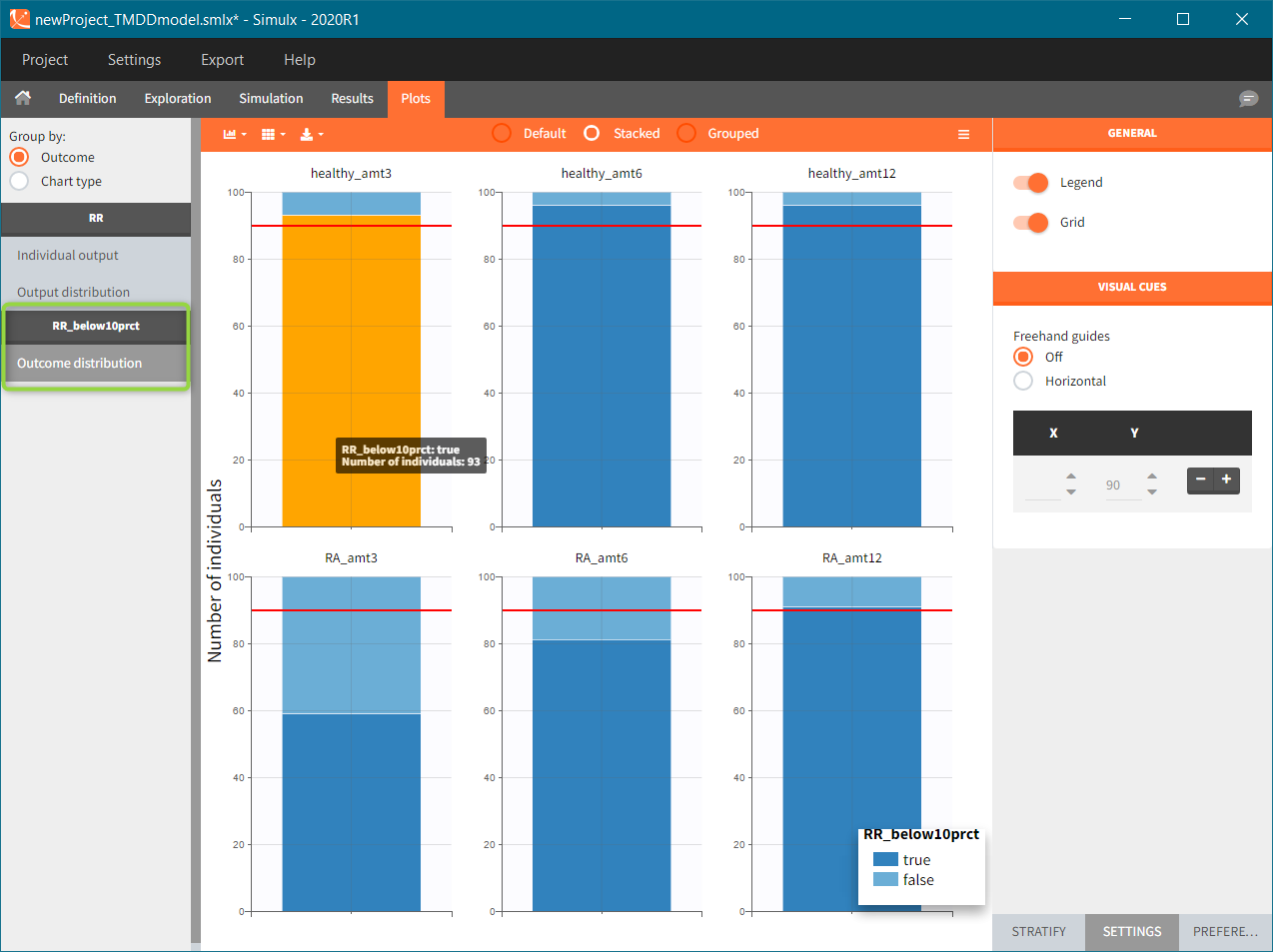
The response at the lowest dose level by healthy individuals is the reference. Group comparison considers a test group a “success” if the odds ratio of “percentage true” is larger then 0.6. Only the highest dose level satisfies this criterion for unhealthy patients.
2.Definition
Exploration or simulation scenarios are build from elements, such as model, parameters, treatments etc. Definition tab, as the name suggests, allows to create these simulation elements through user-friendly and flexible methods. Moreover, it displays them is dedicated sections, which gives a clear overview of the project status. Definition of the following simulation elements is available (click on any of them to see the full description):
- Model
- Occasions
- Population parameters
- Individual parameters
- Covariates
- Treatments
- Outputs
- Regressors
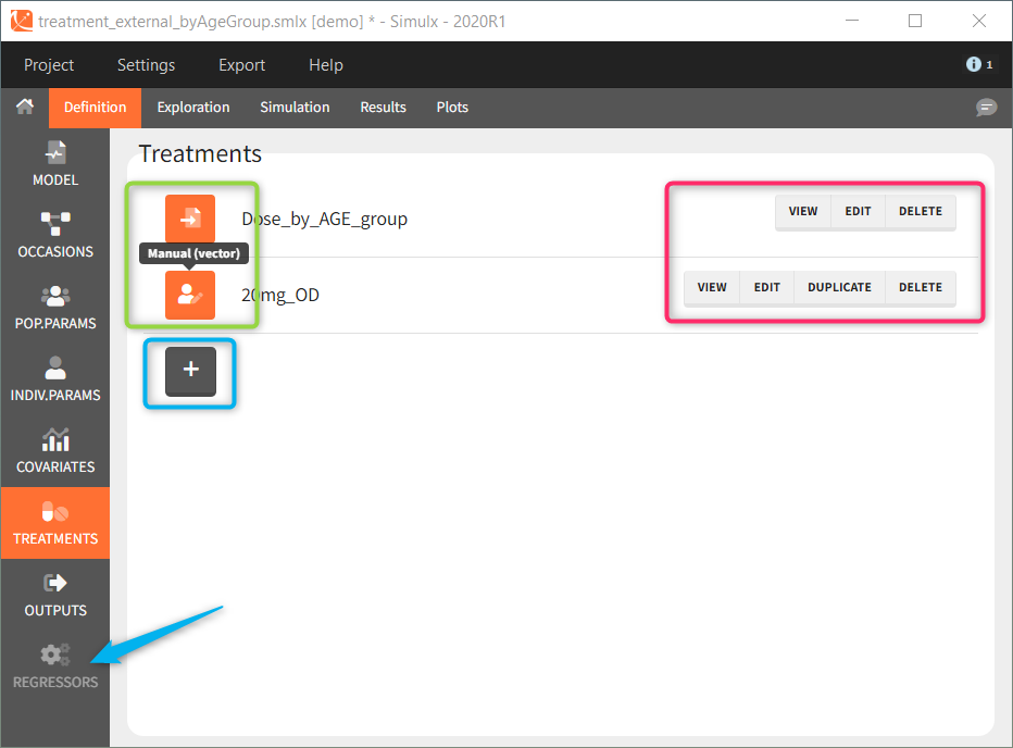
Each element, imported from Monolix or used-defined, is a table ![]() , vector
, vector ![]() or a distribution
or a distribution ![]() . These icons next to the element name inform about the type when you hover on it with a cursor (green frame). Elements can be displayed, edited, duplicated (besides tables) or deleted (red frame). To create a new element, go to a dedicated section and click the “plus” button (blue frame).
. These icons next to the element name inform about the type when you hover on it with a cursor (green frame). Elements can be displayed, edited, duplicated (besides tables) or deleted (red frame). To create a new element, go to a dedicated section and click the “plus” button (blue frame).
Model is a mandatory element. It has to be loaded as first, because only elements present in the model can be defined. Otherwise, the section is greyed out and unavailable, for instance “regressors” (blue arrow at the bottom). Of course, more then one element of each category is possible.
After importing a project from Monolix, all elements are automatically created using Monolix model, results and dataset, see the list of elements here. In a new project written from scratch, Simulx generates default elements based on the loaded model to guide building new ones.
2.1.Model
A single model must be defined in each Simulx project. This model is used both in Exploration and Simulation. Loading or reloading a model deletes all definition elements to avoid incompatibilities between previously defined elements and the new model.
- Model sections:
- [LONGITUDINAL]
- [INDIVIDUAL]
- [COVARIATE]
- Loading or modifying a model
- Model imported from Monolix
- Additional lines
Model sections
The model includes different sections:
- [LONGITUDINAL] (mandatory)
This section contains the structural model. All variables of the model can be defined as outputs of the simulation.
Details on the syntax to define the structural model is here.
This section can include the definition of random variables in a block DEFINITION:, such as a random event or a variable with residual error.
- [INDIVIDUAL] (optional)
If the model considers the inter-individual variability, then definitions of models for individual parameters are in [LONGITUDINAL]. The inputs of [INDIVIDUAL] are population parameters and covariates involved in covariate effects. If the project is imported from Monolix, this section is created automatically. However, when building a project from scratch, the [INDIVIDUAL] section can be generated automatically starting with version 2024 by clicking “+ ADD INDIVIDUAL”. This will add an [INDIVIDUAL] section with all parameters in the model with a lognormal distribution and random effects.
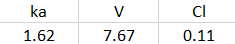
Example: Parameters Tlag, ka, V and Cl are described with lognormal distributions, effects of covariates SEX and logtAGE are included on Tlag and Cl, respectively, and there is a correlation between eta_V and eta_Cl:
[INDIVIDUAL]
input = {Tlag_pop, ka_pop, omega_ka, V_pop, omega_V, Cl_pop, omega_Cl, F_pop, omega_F,
corr_V_Cl, logtAGE, beta_Cl_logtAGE, SEX, beta_Tlag_SEX_M}

SEX = {type=categorical, categories={F, M}}

DEFINITION:
Tlag = {distribution=logNormal, typical=Tlag_pop, covariate=SEX, coefficient={0, beta_Tlag_SEX_M}, no-variability}
ka = {distribution=logNormal, typical=ka_pop, sd=omega_ka}
V = {distribution=logNormal, typical=V_pop, sd=omega_V}
Cl = {distribution=logNormal, typical=Cl_pop, covariate=logtAGE, coefficient=beta_Cl_logtAGE, sd=omega_Cl}
F = {distribution=logitNormal, typical=F_pop, sd=omega_F}
correlation = {level=id, r(V, Cl)=corr_V_Cl}
More details on the syntax in this section is here.
- [COVARIATE] (optional)
If covariates are used in the model of individual parameters, then they should be defined in a block [COVARIATE]. This block contains the list of inputs (covariates used in the model) and the definition of categories for categorical covariates. It can also include transformations of the covariates, in a section EQUATION: for continuous covariates and in a section DEFINITION: for categorical covariates. All the covariates defined in this block (transformed or not) can be then used in the block [INDIVIDUAL].
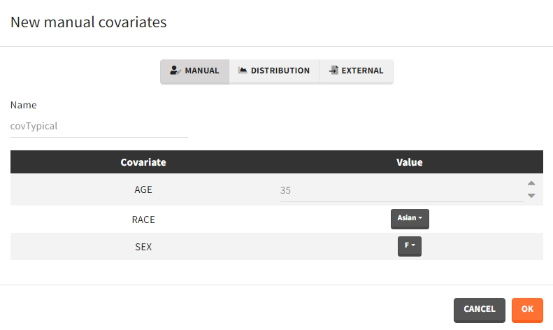
Example: There are 3 covariates AGE, RACE and SEX. The covariate AGE is transformed into logtAGE, RACE is transformed into tRACE.
[COVARIATE]
input = {AGE, RACE, SEX}

RACE = {type=categorical, categories={Asian, Black, White}}
SEX = {type=categorical, categories={F, M}}

EQUATION:
logtAGE = log(AGE/35)

DEFINITION:
tRACE =
{
transform = RACE,
categories = {
G_Asian = Asian,
G_Black_White = {Black, White} },
reference = G_Black_White
}
More details on the syntax in this section is here.
Note that in Simulx it is not possible to define covariates as distributions within the block [COVARIATE] with a section DEFINITION:. However, the covariate distributions can be defined in the tab Definition in the interface of Simulx.
Loading or modifying a model
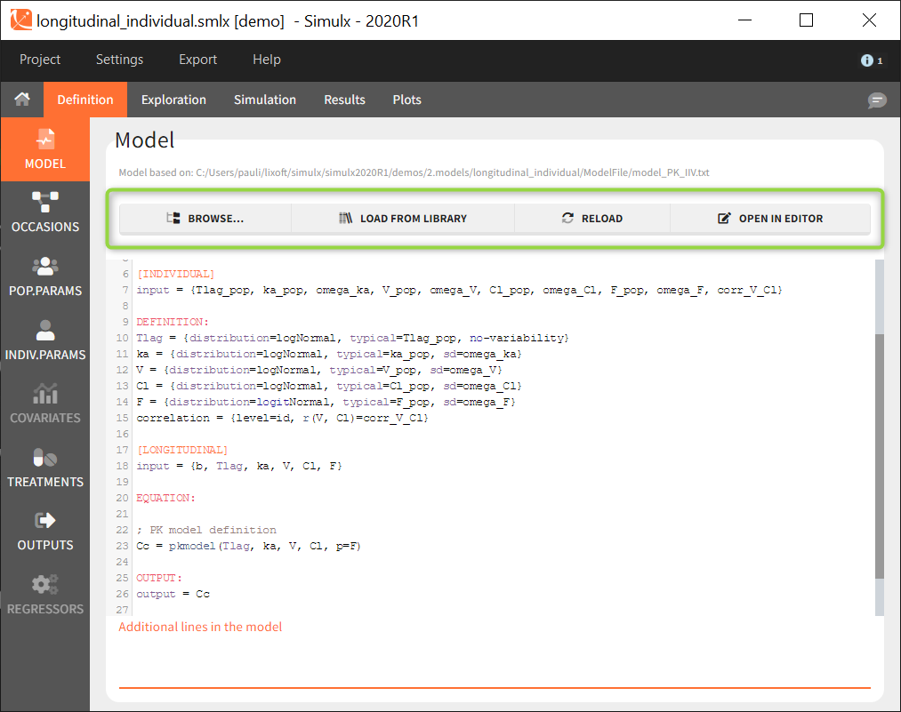
Several buttons are available on the top of the page to load or modify a model:
- Browse: to load a new model file by browsing if from the computer.
- Load from library: to load a model from the built-in libraries. Note that all models from the libraries contain only structural models ([LONGITUDINAL] block) with no individual models for the parameters or covariates.
- Reload: to reload the same model after modifying it using the built-in editor or with any text editor.
- Open in editor: to opens the current model in the built-in editor.
Loading or updating a model with the buttons “Browse”, “Load from library” or “Reload” deletes all definition elements to avoid incompatibilities with previously defined elements and the new model.
Model imported from Monolix
When importing a model from Monolix, the model that appears in the interface of Monolix comes from two sources:
- The structural model ([LONGITUDINAL] block) used in the Monolix project, copied in a new file stored in the result folder of the Simulx project, in a subfolder names ModelFile/.
- The [INDIVIDUAL] and (if there are covariates in the model) [COVARIATE] blocks, derived from the statistical model set up in Monolix, saved directly in the .smlx file.
Warning: When opening a model in the editor with “Open in editor”, only the new structural model file is opened for modifications. If this model is changed and reloaded, it will replace the two model sources mentioned above. It means that the [INDIVIDUAL] and [COVARIATE] blocks are removed. To keep these blocks in the modified model, they have to be pasted in the file together with the [LONGITUDINAL] block.
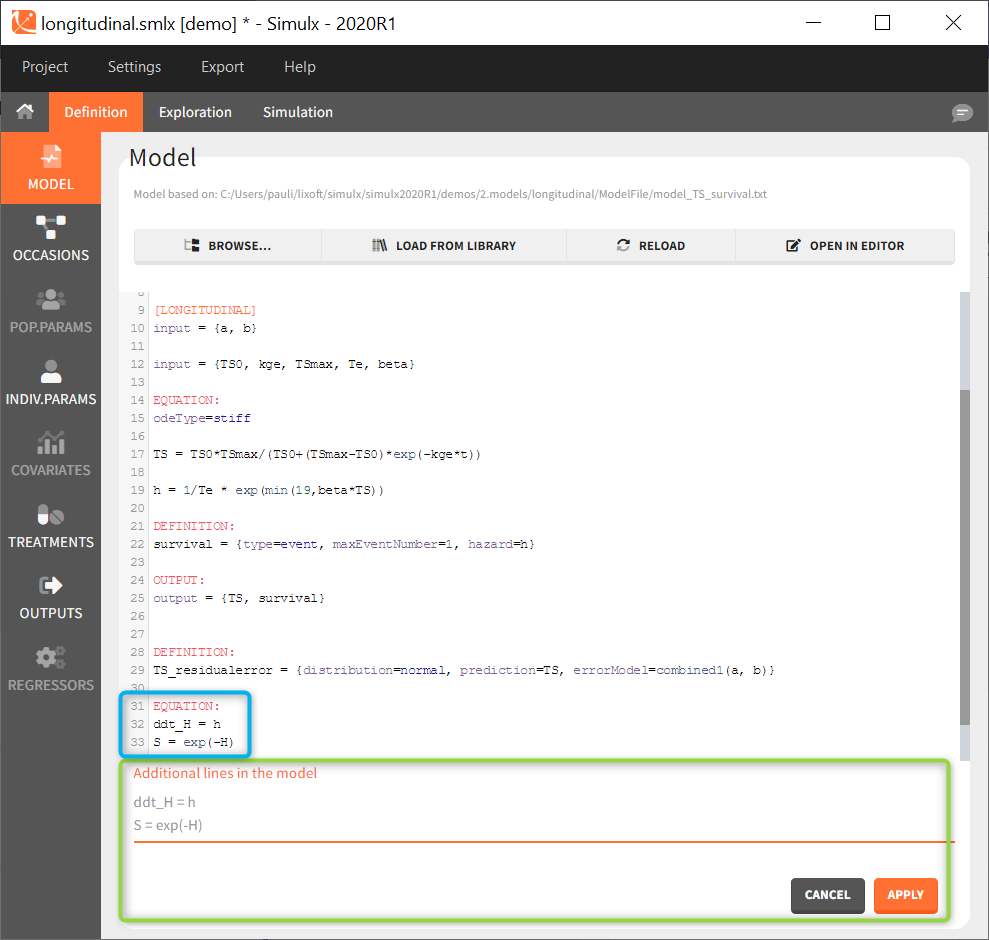
Additional lines
Below a model definition, there is a field to write additional lines, which are included “on the fly” in the model. Note that in version 2024 and later, this is accessed by clicking the button “+ ADD LINES”.
This is convenient for example to use variables for simulations that are not defined in the Mlxtran model code, such as the AUC, a change from baseline, or the survival function (see example below). The model file itself is not modified, the additional lines are saved in the .smlx file.
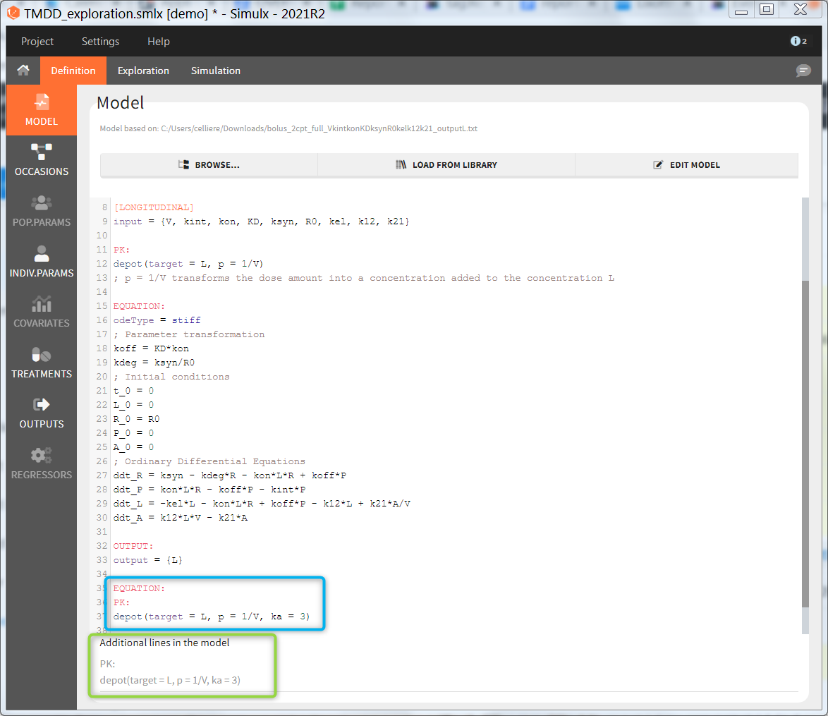
By default, the additional lines are added in a new section EQUATION: below the structural model. In order to add additional lines in the PK block, it is necessary to add “PK:” at the beginning of the additional lines. This is convenient to add a new route of administration, using the iv(), oral() or depot() macro for instance. If this new administration depends on a parameter (e.g the absorption rate ka), the parameter needs to be fixed in the additional lines. It cannot be added to the input parameter list. It is not possible to add additional lines in the [INDIVIDUAL] or [COVARIATE] blocks.
This function is available also with lixoftConnectors functions: setAddLines() and getAddLines(), see here for more details.
Warning: When using “import from Monolix”, “additional lines” fields can (sometimes) be unavailable. In this case, open the Monolix project in Monolix and use “Export to Simulx”. This problem has been fixed in the 2021R1 version.
In the example below, a oral absortion route in added to the demo TMDD_exploration.smlx, which originally had only iv:
2.2.Occasions
Occasions definition. When the model to simulate contains inter-occasion variability (ie variability between different periods of measurements within the same individual), you should define a single element Occasions. Like for the model, and contrary to the other simulation elements, it is not possible to define several occasion elements to choose from for the simulation.
Demo projects: 3.7. occasions
All other defined elements must be compatible with the structure of occasions.
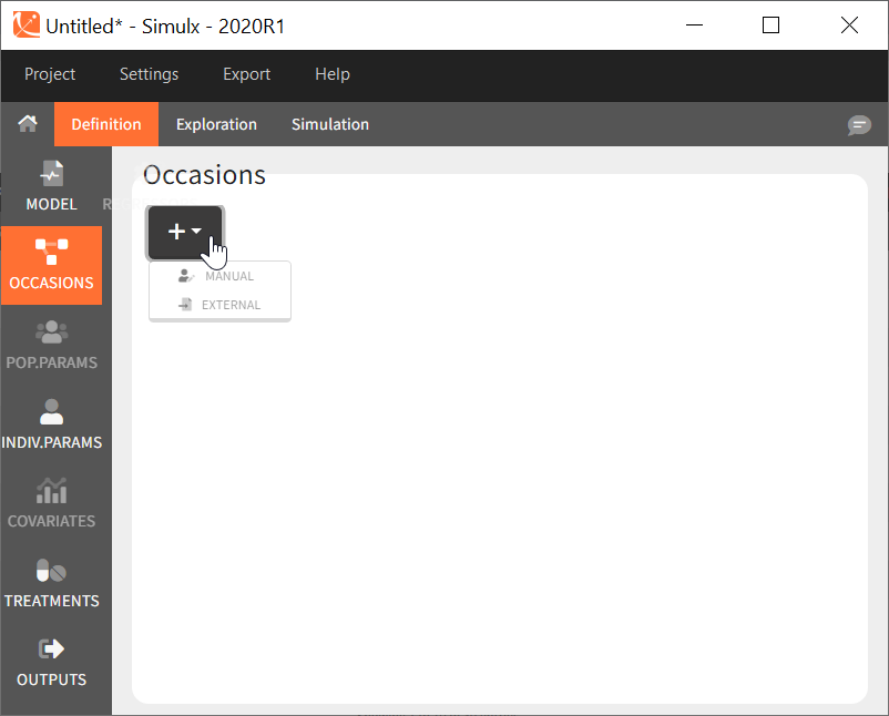
Common occasions for all subjects
In the interface, it is possible to define a common structure of occasions applied to all simulated subjects. This structure can contain one or several levels of occasions, and one or several occasions per subject.
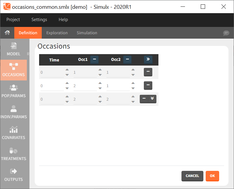
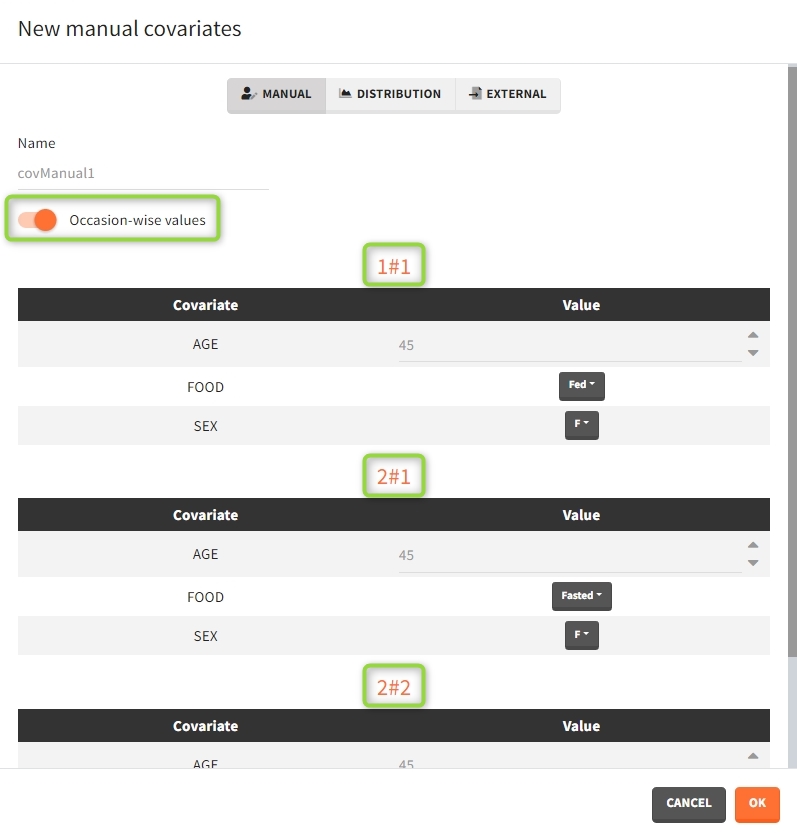
After defining such common occasion structure, other common elements (parameters, covariates, treatments, outputs and regressors of type “manual” or “regular”) can be defined occasion-wise thanks to a dedicated toggle “occasion-wise values”, as on this example screenshot for covariates:
Moreover, elements defined as external tables may contain one or several columns to assign different values to different subject-occasions.
Subject-specific occasions
To define subject-specific occasions use an external file containing a table with columns ID, time and one or several columns for the occasions. The header names for these columns are free and are used by Simulx. The external file separator can be tab, comma or semicolon. The possible file extensions are .csv or .txt.
Below is an example of the occasions element defined after loading the external table (on the left).
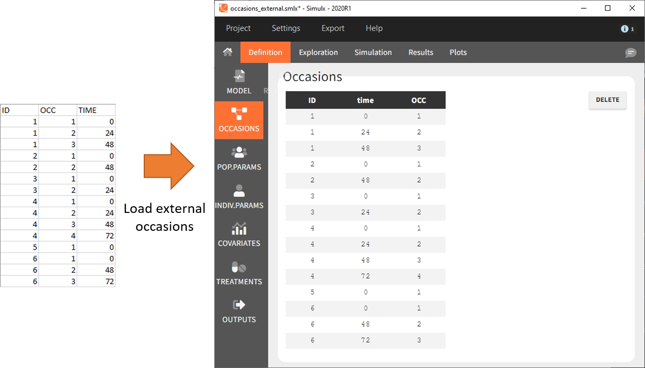
After defining such subject-specific occasion structure, other elements (parameters, covariates, treatments, outputs and regressors) must be common over subjects (type “manual”, “regular” or “distribution”), or can be defined with occasion-wise values as external tables only, with the same occasion structure.
Occasions imported from Monolix
Upon import of a Monolix run, Simulx creates an occasion element with the individual structure of occasions from the Monolix data set.
- mlx_subjects: a table containing the occasions and their starting times for each individual. The table has at least 3 columns: id, time, occ. Additional columns may be present in case of several levels of occasions.
Rules for simulating occasions
- Occasions are not simulated in Exploration: only the first occasion from the selected subject is simulated.
- If occasions are not defined, inter-occasion variability is not taken into account for the simulation of individual parameters.
- From the 2023 version on, the sampling of individual parameters takes into account the inter-occasion variability if one or several occasions are defined. In previous versions (2020 and 2021), if the structure of occasions contains a single occasion for some subject, then the simulation of individual parameters for this subject does not take into account inter-occasion variability.
- When an occasion element has been defined, in case of several replicates, the sampling method has to be ‘Keep Order’.
Occasions in outcomes, results and plots
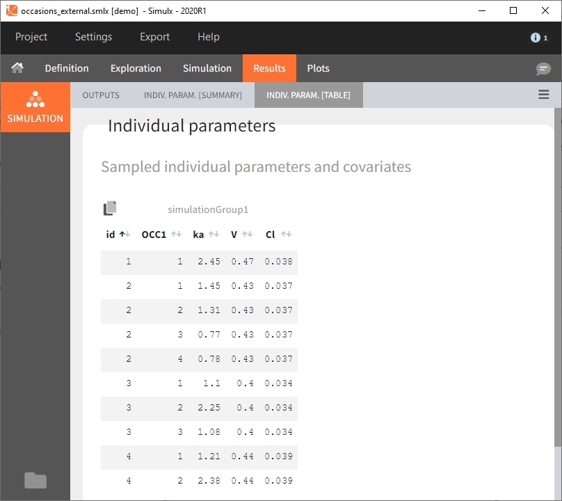
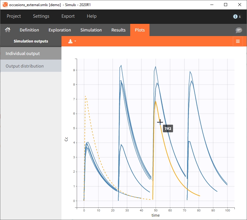
Occasions are indicated as additional columns in the table of individual parameters. In the plots of individual outputs, occasions are highlighted as dashed yellow lines on hover of one the occasions from the same subject. Furthermore, all plots of results can be stratified by occasions.
When occasions are defined, the definition of outcomes can be made by post-processing the simulation outputs by subject (one outcome value per individual) or by subject-occasion (one outcome value for each occasion of each individual). When the post-processing by subject-occasion is selected, the occasion column(s) appear(s) also in the corresponding outcome table.
2.3.Population parameters
Definition of population parameters as simulation elements allows to simulate individual parameters from probability distributions. In the mlxtran model they are:
- [INDIVIDUAL] block input parameters that are neither inputs nor outputs of the block [COVARIATE].
- [LONGITUDINAL] block input parameters that are neither individual parameters nor regressors.
POP.PARAM section in the “Definition” tab is available only if the list of population parameters from the model is not empty.
Demo projects: 3.3. population parameters
Overview
In the “Population parameters” tab, elements created automatically after a “new project” or an “import from Monolix/PKanalix” and elements created by the user are shown.
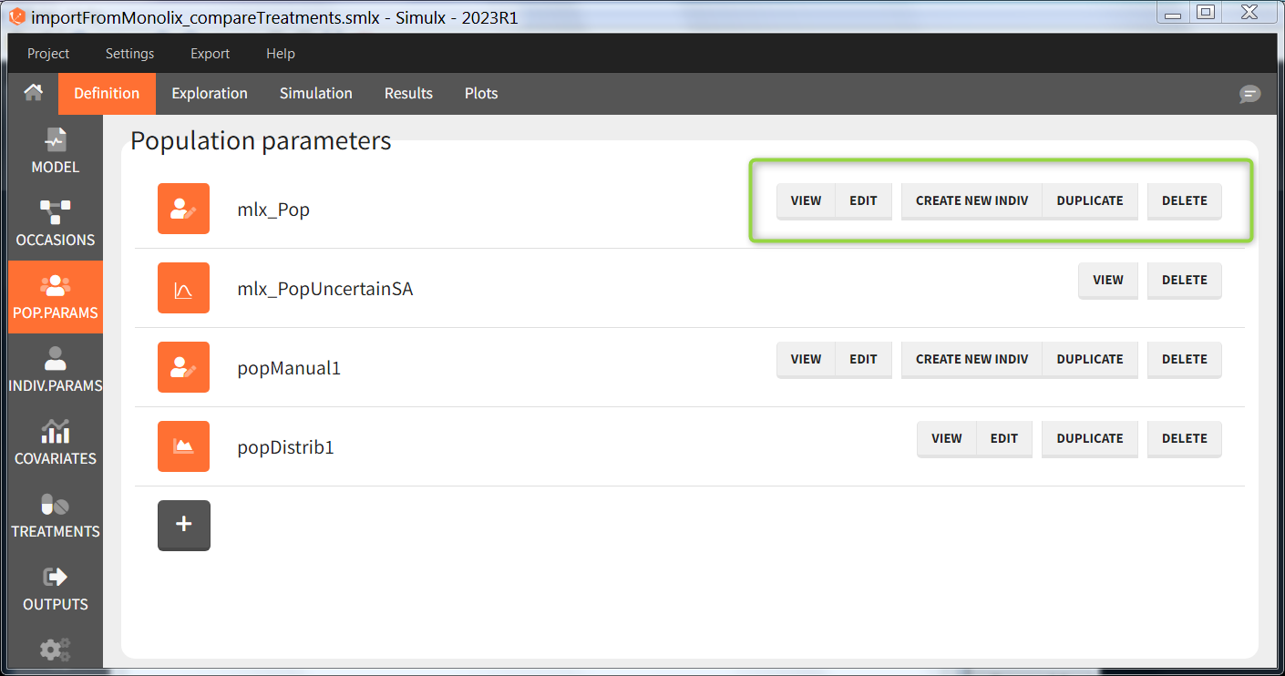
The buttons on the right allow to do the following actions:
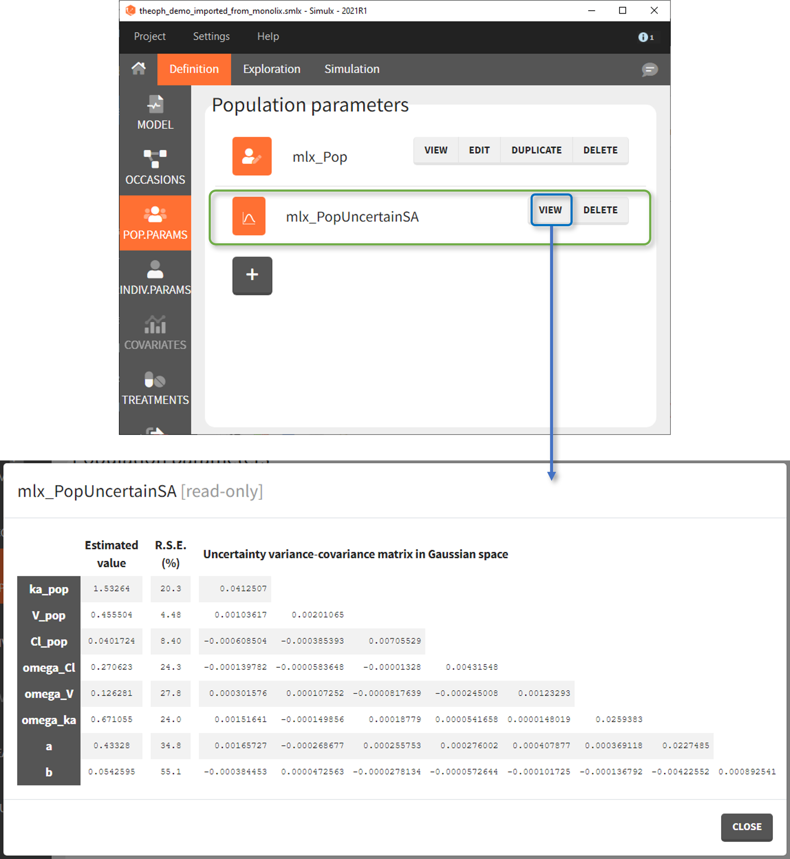
- VIEW: display the content of the element (the value of the population parameters)
- EDIT: modify the content of the element. Note: the elements “mlx_PopUncertainSA”, “mlx_PopUncertainLin”, “mlx_TypicalUncertainSA”, and “mlx_TypicalUncertainLin” represent multidimentional distributions and cannot be edited.
- DUPLICATE: open a pop-up window for a new element with the same content as the previous element. Note: the elements “mlx_PopUncertainSA”, “mlx_PopUncertainLin”, “mlx_TypicalUncertainSA”, and “mlx_TypicalUncertainLin” cannot be duplicated. Elements based on external files can also not be duplicated.
- DELETE: delete the element. When the deleted element is based on an external file located in <result folder>/ExternalFiles, the file itself is also deleted upon save.
- CREATE NEW INDIV: creates a new element “individual parameters” from the population parameters fixed effects (e.g V = V_pop). This option is available for population elements of type “manual” only.
New population parameters element
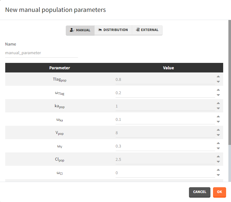
After loading a model, Simulx generates automatically a default population parameter element. It is a table with parameters names from the model and all entries equal to one. It helps to create a new element by just modifying the values. Clicking the button “plus” adds a new population parameter, which may be one of the three types.
- Manual: It is a vector and has one value for each parameter.
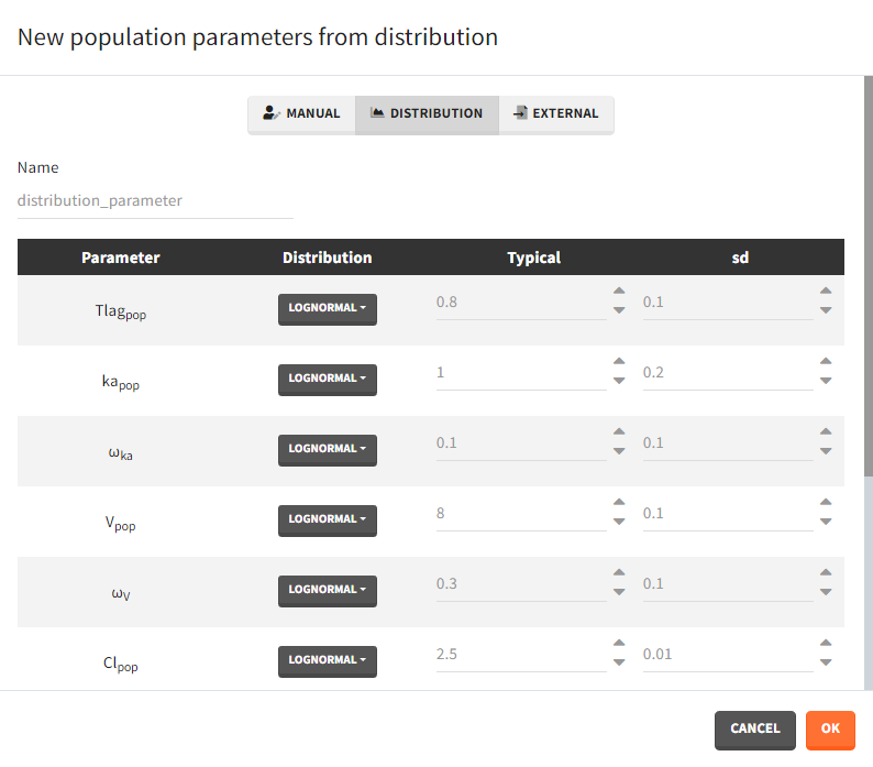
- Distribution: Parameters are a distribution law – normal, lognormal (default), logitnormal, uniform – with a typical value and a standard deviation. If the distribution is lognormal or logitnormal, sd is the standard deviation of the distribution in the Gaussian space. The typical value is the median of the population parameter distribution. In the case of a lognormal distribution, in order to get the sd \(s_G\) of the distribution in the Gaussian space given a typical value of the lognormally distributed covariate \(\mu\), or given its mean \(m\), and given its sd \(s\), you can use the following formulae:\[s_G = \sqrt{\ln\Big(1+\Big(\frac{s}{m}\Big)^2\Big)} = \sqrt{\ln\Bigg(1+\sqrt{1+4\Big(\frac{s}{\mu}\Big)^2}\Bigg) – \ln(2)}\]Both formulae are equivalent if \(\frac{s}{\mu}<<1\) (in that case \(\mu \approx m\)).
- External: It is a file with a table that has each population parameter in a separate column.
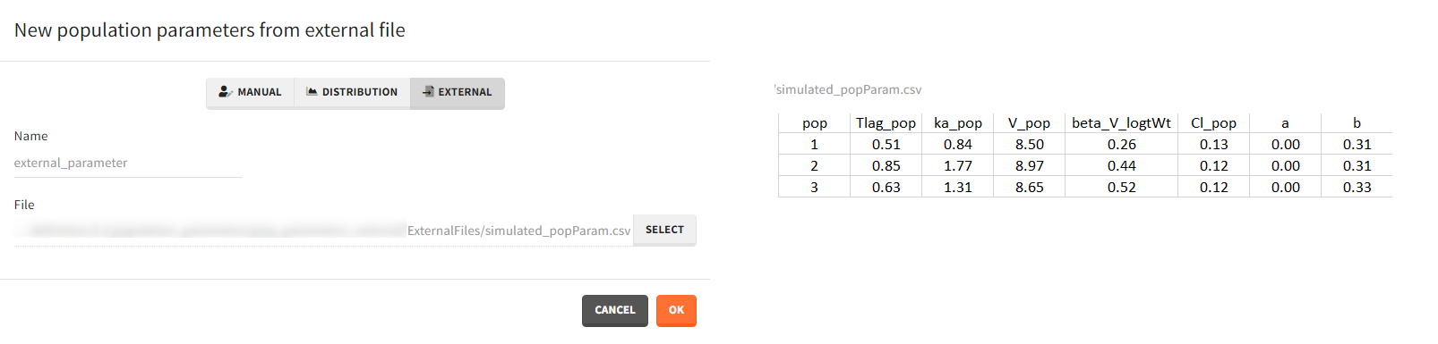
The external file can have only one column header different from the population parameters names. It indicates replicates (eg. from bootstrap or simpopmlx). All individual parameters of the same replicate come from the same population distribution.
Population parameters imported from Monolix
Demo projects: 1.overview/importFromMonolix … .smlx
Importing a Monolix project generates automatically a population parameter element with values from the Monolix result folder.
- mlx_Pop contains population parameters estimated by Monolix if the POP.PARAM task results are available.
- mlx_PopInit contains initial estimates of the population parameters if the mlx_pop does not exist.
- mlx_Typical (NEW since 2023 version) is the same as mlx_Pop but with all standard deviations of random effects (omega parameters) set to 0. It enables to simulate a typical individual in terms of parameters (no unexplained variability), and still include non-typical covariates in the simulation. The variability in the sampled individual parameters will come only from sampling different covariate values. To see how this element can be used in practice, check the demo project 1.overview/importFromMonolix_CovEffectOnTypical.smlx.
mlx_Pop, mlx_PopInit and mlx_Typical are vectors (single set of population parameters). If replicates are used in the Simulation tab, with these elements, the same set of poplation parameters will be used for all replicates.
- mlx_PopUncertainSA (resp. mlx_PopUncertainLin) enables to sample population parameters using the variance-covariance matrix of the estimates computed by Monolix if the Standard Error task (Estimation of the Fisher Information matrix) was performed by stochastic approximation (resp. by linearization). To sample several population parameter sets, this element needs to be used with replicates. In the interface, the element is displayed with a reminder of the estimated values and RSEs next to the variance-covariance matrix which is used to generate new samples.
The displayed variance-covariance matrix and the sampling is done in the gaussian space (i.e we sample {log(V_pop), log(Cl_pop), omega_V, omega_Cl, b} from a multivariate normal distribution, if V and Cl have a lognormal distribution). The sampled values are then converted to the non-gaussian space. For omega and error parameters, negative samples values are rejected, they are thus sampled from truncated normal distributions.
This element cannot be modified nor duplicated.
- mlx_TypicalUncertainSA (resp. mlx_PopUncertainLin, NEW since 2023 version) is another population parameter element with the variance-covariance matrix of population parameter values estimated in Monolix. The only difference to the previous mlx_PopUncertainSA/Lin is that it has standard deviations of random effects (omega parameters) set to 0. It enables to simulate a typical individual with different typical parameter values for each replicate, such that the uncertainty of parameters is propagated to the predictions. To sample several parameter sets, this element needs to be used with replicates. To see how this element can be used in practice, check the demo project 1.overview/importFromMonolix_UncertaintyOnTypical.smlx.
In the following video we apply uncertainty on fixed effects only (with version 2021). With the 2023 version, the steps performed outside of the interface in this video can all be replaced by simply selecting the new element mlx_TypicalUncertain.
2.4.Individual parameters
In the mlxtran model, the following parameters are recognized as individual parameters:
- Only the [LONGITUDINAL] block is present: all parameters of the input list, except those defined as regressors.
- Both the [LONGITUDINAL] and [INDIVIDUAL] blocks are present: parameters defined in the DEFINITION section of the [INDIVIDUAL] block.
Individual parameters can be used in the tab “Exploration” and “Simulation”. An individual parameter definition is either a vector, which has one value per parameter, or a table, where each line correspond to a value of a different individual.
Demo projects: 3.4. individual parameters
Overview
In the “Invidual parameters” tab, elements created automatically after a “new project” or an “import from Monolix/PKanalix” and elements created by the user are shown.
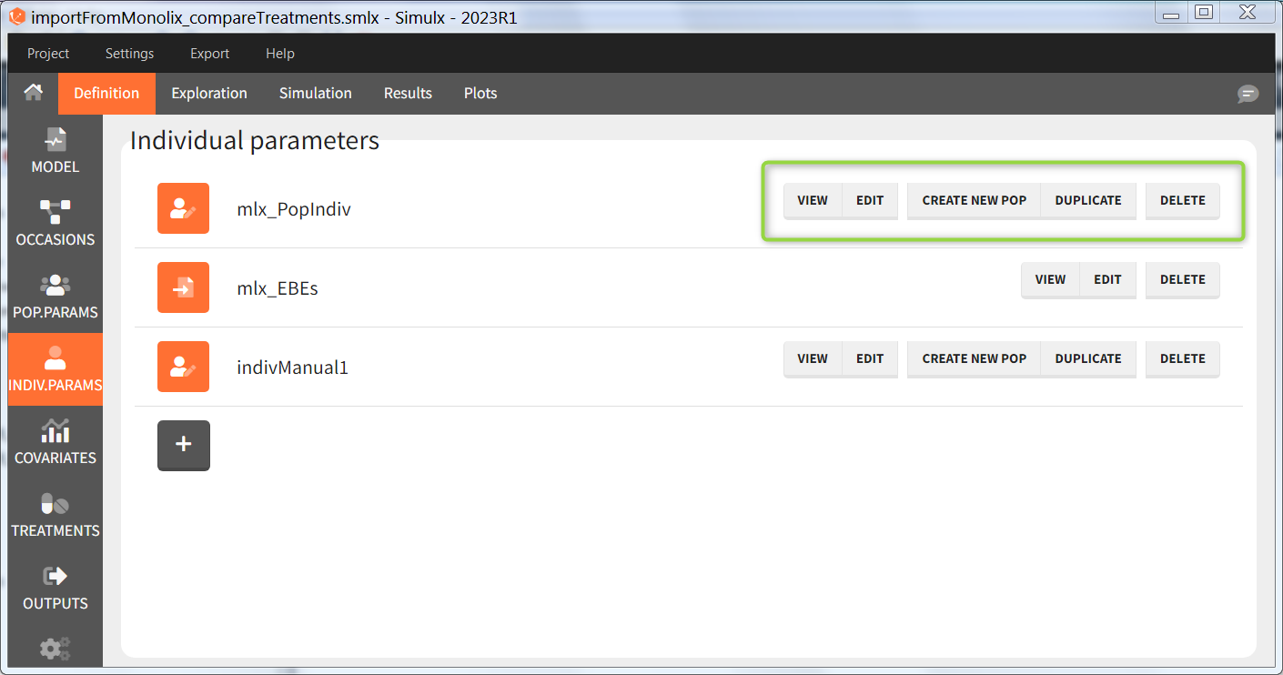
The buttons on the right allow to do the following actions:
- VIEW: display the content of the element (the value of the individual parameters)
- EDIT: modify the content of the element.
- DUPLICATE: open a pop-up window for a new element with the same content as the previous element. Note: elements based on external files cannot be duplicated.
- DELETE: delete the element. When the deleted element is based on an external file located in <result folder>/ExternalFiles, the file itself is also deleted upon save.
- CREATE NEW POP: creates a new element “population parameters” from the individual parameters (e.g V_pop = V). The betas (covariate effects), omegas (standard deviation of the random effects), correlation and error parameters are set to zero. This option is available for individual elements of type “manual” only, which contain a single set of individual parameters.
New individual parameters elements
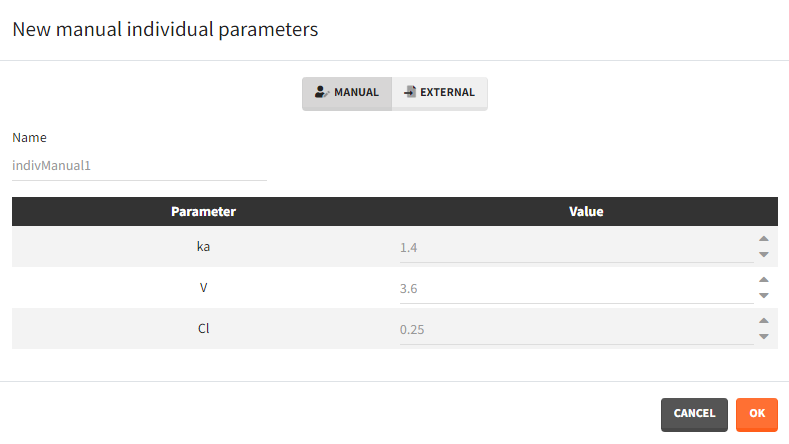
After loading a model, Simulx generates automatically a default individual parameter element called “IndivParameters” with all values set to 1. This element can be modified (button EDIT). New elements can be created with the button “+”. Two different types of individual parameter elements are available:
- Manual: One value per parameter to type in. The required parameters are automatically listed.
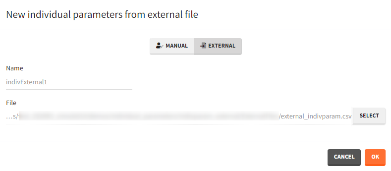
- External: An external text file with either:
- A single row and one column per parameter. The headers must correspond to the parameter names.
- Several rows, a first column with header “id”, occasion columns (optional) and one column per parameter. The headers must correspond to the parameter names, and to the occasion names if applicable.

- A single row and one column per parameter. The headers must correspond to the parameter names.
The external file can be tab, comma or semicolon separated. Available file extension are: .csv or .txt.
Individual parameters elements imported from Monolix
Upon import of a Monolix run, several individual parameters elements are created automatically:
- mlx_IndivInit: [when POP.PARAM task has not run]a vector of individual parameters corresponding to the initial values of the population parameters in Monolix, i.e with covariate betas and random effects set to zero. For instance, \( V=V_{pop,ini} \)
- mlx_PopIndiv: [when POP.PARAM task has run]a vector of individual parameters corresponding to the population parameters estimated by Monolix, i.e with covariate betas and random effects set to zero. For instance, \( V=V_{pop,est} \)
- mlx_PopIndivCov: [when POP.PARAM task has run and covariates are defined in the Monolix data set]a table of individual parameters corresponding to the population parameters and the impact of the covariates, but random effects set to zero. For instance, \( V=V_{pop} \times \left( \frac{WT}{70} \right) ^{\beta_{V,WT}} \)
- mlx_EBEs: [when EBEs task has run] a table of individual parameters corresponding to the EBEs (conditional mode) estimated by Monolix (as displayed in Monolix Results > Indiv. param > Cond. mode.)
- mlx_CondMean: [when COND. DISTRIB. task has run] a table of individual parameters corresponding to the conditional mean estimated by Monolix (as displayed in in Monolix Results > Indiv. param > Cond. mean.)
- mlx_CondDistSample: [when COND. DISTRIB. task has run] a table of individual parameters corresponding to one sample of the conditional distribution (first replicate of the Monolix result file IndividualParameters/simulatedIndividualParameters.txt).
2.5.Covariates
Values to use for simulation should be defined for covariates used in the statistical model, if the simulation is based on population parameters. In this case, new individual parameters are simulated from the population distributions and the covariate values. Several covariate elements can be defined in Definition, but only one covariate element should be used per simulation group in Simulation. No covariate element can be used in Exploration, since only individual parameters are used in Exploration.
Demo projects: 3.2. covariates
New covariate element
Several types of covariate elements can be defined:
- Manual: It is a vector that has one or several dosing times with identical or different amounts. The + and – buttons allow to add and remove doses.
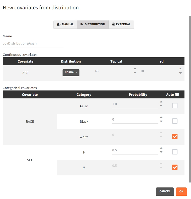
- Distribution: The covariates are described with distribution laws. When this type of element is used for simulation, new covariate values are simuated from the distributions. For continuous covariates, the distribution can be normal, lognormal or logitnormal with a mean and sd, or uniform with two interval limits. If the distribution is lognormal or logitnormal, sd is the standard deviation of the distribution in the Gaussian space. The typical value is the median of the covariate distribution..
 In the case of a lognormal distribution, in order to get the sd \(s_G\) of the distribution in the Gaussian space given a typical value of the lognormally distributed covariate \(\mu\), or given its mean \(m\), and given its sd \(s\), you can use the following formulas:
\[s_G = \sqrt{\ln\Big(1+\Big(\frac{s}{m}\Big)^2\Big)} = \sqrt{\ln\Bigg(1+\sqrt{1+4\Big(\frac{s}{\mu}\Big)^2}\Bigg) – \ln(2)}\]
Both formulas are equivalent if \(\frac{s}{\mu}<<1\) (in that case \(\mu \approx m\)).
For categorical covariates, the probability for each category can be defined in [0,1]. The sum of probabilities over all categories must be 1, and an “auto fill” option allows to automatically fill one or several of the categories to satisfy this rule.
- External: An external text file with columns id (optional), occasions (optional), and one column per covariate (mandatory). The occasions headers must correspond to the occasion names defined in the occasion element. When id and occasion columns are present, then they must be the first columns. When the id column is not present, the covariate is considered ‘common’, i.e the same for all individuals. Categorical covariate values must correspond to the categories defined in the model (block [COVARIATE]).The external file can be tab, comma or semicolon separated. The possible file extensions are .csv or .txt.
Covariate elements imported from Monolix
Importing a Monolix project generates automatically a covariate element based on the Monolix data set.
- mlx_Cov: contains covariate information for each individual. The table is saved as external table in the result folder of the project. This table contains a column id, and one column per covariate. If there are occasions in the Monolix project, it also contains one or several columns for the occasion levels.
- mlx_CovDist: element of type “distribution” with typical values, standard deviations and probabilities calculated on the individuals of the Monolix project. No correlation between the covariates is assumed. In the 2020 version, all continuous covariates are assumed to follow a normal distribution. In the 2021 version, continuous covariates having only strictly positive values in the Monolix data set are assumed to follow a log-normal distribution, and the others are set with a normal distribution.
2.6.Treatments
Treatments definition includes times and amounts of the doses applied to the model. Treatments are applied to the model via the macros depot(), iv() or oral() used in the model. Moreover, treatments definition has an administration id, which allows to choose to which macros used in the model the doses are applied.
When used in “Exploration” or “Simulation“, several treatment elements can be combined together. For instance, a loading dose of type manual followed by maintenance doses of type regular, or a oral dose with adm=2 and an iv dose with adm=1.
The units of time and amounts must be consistent with the units of the Monolix data set or with the model definition when starting from scratch.
Demo projects: 3.1. treatments
New treatments element
Several types of elements can be defined:
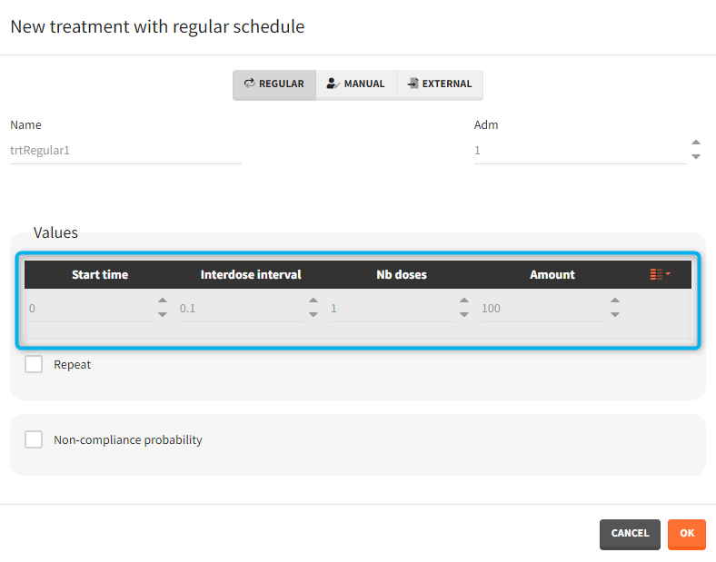
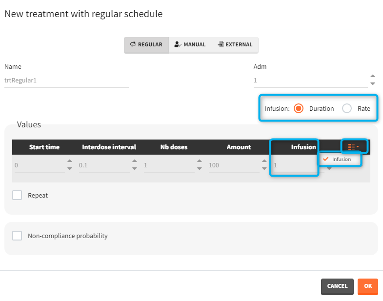
- Regular: It is used for regularly spaced dosing times with a unique amount and a unique infusion duration or rate (optional). It requires the start time, inter-dose internal, number of doses, and amount.
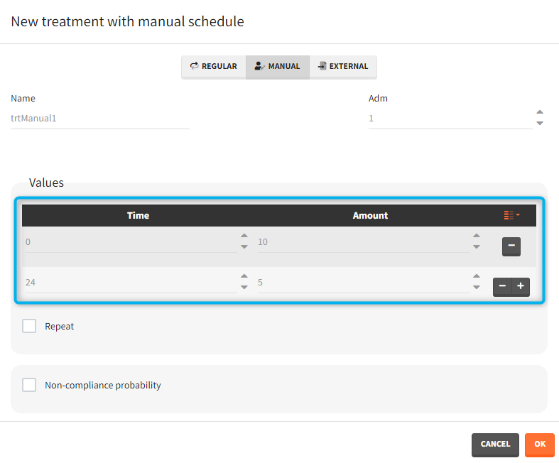
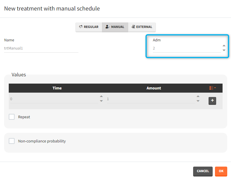
- Manual: It is a vector that has one or several dosing times with identical or different amounts. The + and – buttons allow to add and remove doses.
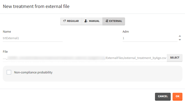
- External: An external text file with columns id (optional), occasions (optional), time (mandatory), amount (mandatory), tinf or rate (optional), washout (optional). The occasions headers must correspond to the occasion names defined in the occasion element. When id and occasion columns are present, then they must be the first columns. When the id column is not present, the treatment is considered ‘common’, i.e the same for all individuals. The washout column can contain zeros (no washout) or ones (washout).
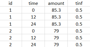
The external file can be tab, comma or semicolon separated. The possible file extensions are .csv or .txt.
Additional treatments definition specifications:
- adm: [all] the administration id of the treatment element (integer). The doses of a treatment element with adm=2 apply to all model macros defined with adm=2, for instance
oral(adm=2, ka). Macros used in the model without adm are implicitly defined with adm=1.
- infusion duration or rate: [regular/manual] the list button on the right allows to display the infusion column. The value is understood as either a duration or a rate, depending on the chosen option.
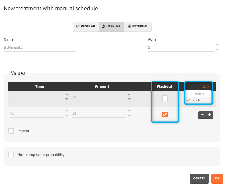
- washout: [manual] the list button on the right allows to display the washout column. When the washout tick-box is selected, a washout is applied just before the dose. A washout means that all model variables are reset to their initial values.
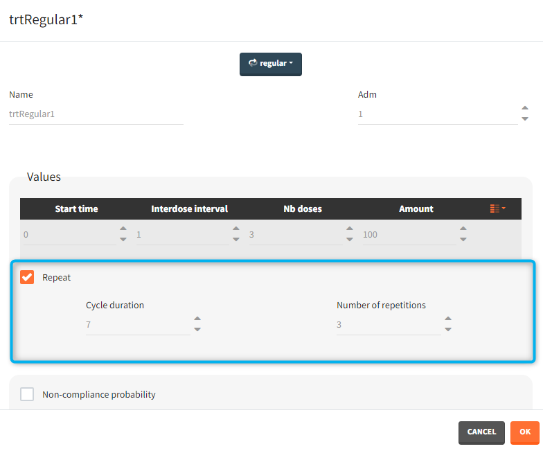
- repeat: [regular/manual] This option allows to repeat a base pattern of doses several times (number of repetitions), with a given periodicity (cycle duration). In the example below, the dose is given on the three first days of the week, for 4 weeks. The doses on the first week are defined using the type ‘regular’ with three doses and an inter-dose interval of 1 day. This base pattern is then repeated every 7 days (cycle duration), 3 times (number of repetitions) in addition to the first week.
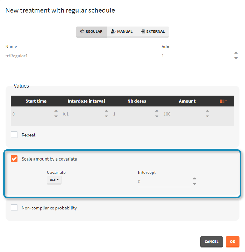
- scale amount by a covariate: [regular/manual] This option allows to personalize the dose given to different individuals by scaling the dose amount with the selected covariate and with a specific intercept for the linear relationship: \(\text{Scaled amount} = \text{Amount} \times \text{Selected covariate} + \text{Intercept}\).
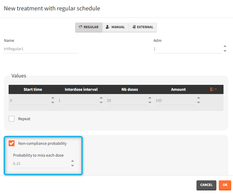
- non-compliance probability: [all] The doses defined are applied to the model with a given probability (1-p) , where p is the probability to miss a dose. This allows to simulate non-adherence to a treatment. Which doses are applied and which are not rely on the random number seed defined in the project settings to ensure reproducibility.
Treatment elements imported from Monolix
Importing a Monolix project generates automatically a treatment element for each administration id defined in the Monolix data set.
- mlx_AdmX: contains treatment information for admID=X for each individual including: dosing times, amount, infusion duration or rates (optional) and washouts (optional, from EVID=3 or EVID=4 in Monolix). The Monolix data set column SS is replaced by additional dose lines as defined by the Monolix setting “number of steady-state doses”. The ADDL column is also replaced by additional dose lines.
2.7.Outputs
Outputs of simulations are variables from the longitudinal model of continuous, discrete or event type. There are two outputs groups:
- Main outputs
- Model predictions defined in the structural model as the “output” (eg. Cc).
- Observations (model predictions with an error model) defined in the observation model (eg. y1).
- All variables defined in the structural model as “tables” (eg. AUC).
- Intermediate outputs
- Variables computed in the structural model and not listed as an “output” or “table” in the OUTPUT block (eg. amount in the peripheral compartment, time varying clearance).
- Regressors.
- Variables defined with the “additional lines” in the model definition.
Loading a model automatically generates the “main outputs”. Model predictions and tables are on a default time grid. If a project is built from scratch, then model observations use also the default time grid. Otherwise, in case of project imported from Monolix, they are on a grid given by the measurement times from the Monolix dataset.
Projects: 3.5.outputs, 7.noncontinuous_outputs
New output element
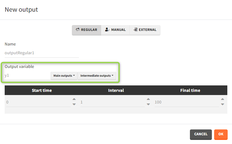
Outputs correspond to output variables, which can be written or selected from the list (green frame).
It is possible to have different outputs of the same variable. For example, one output shows the time evolution over a treatment period and another gives a value at the end of treatment to define an endpoint. However, charts display these outputs on one plot with merged time grids.
There are three output types.
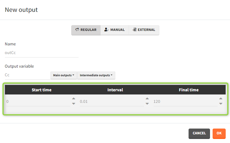
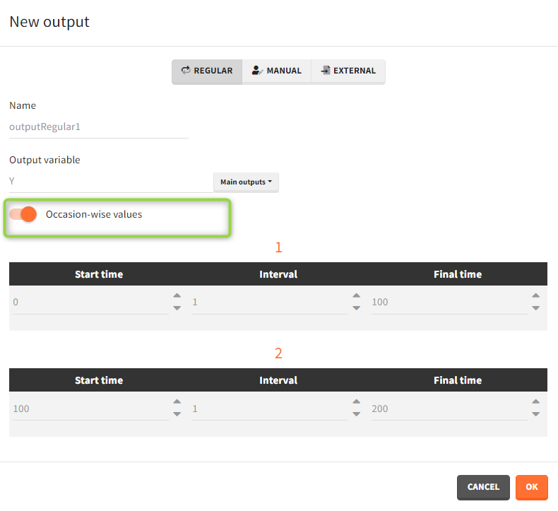
- Regular: It is a vector on a regular time grid (start time, step, final time, (occ)) common for all subjects.
- Manual: It is a vector with manually defined list of time points (use “space” to separate them) common for all subjects.
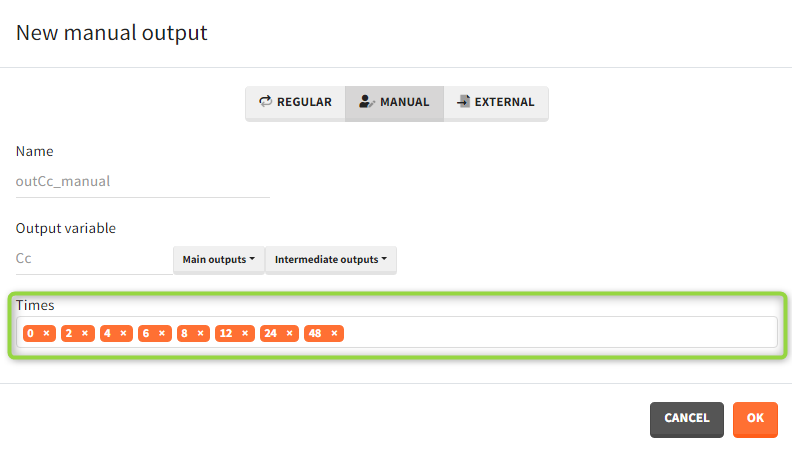
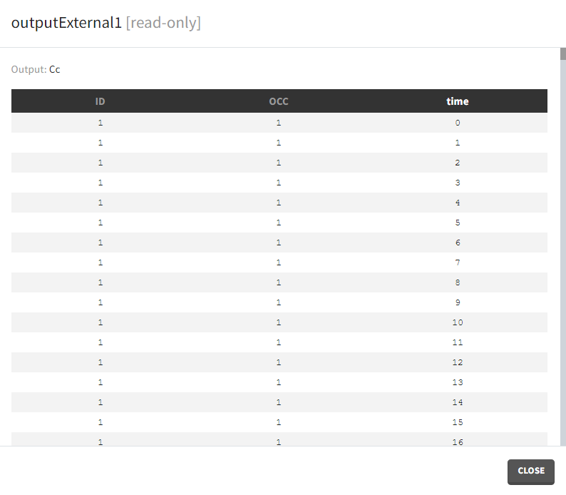
- External: It is a file with a table that has: a mandatory column “time” for time points, an optional column “id” (in the absence of the “id” column the time grid is equal for all subjects), and an optional column “occ” for occasions.
Occasions
By default, the regular and manual output types apply to all subject-occasions. If occasions are common among all individuals, then an option “occasion-wise values” is available. In this case each occasion has a separate time grid.
Time-to-event outputs
Time limits (start time and final time) define the observation period during which the survival curve is computed. The final time thus defines the censoring time. Intermediate times are ignored. The time grid must be the same for all individuals. If an external file is provided with different start and end values for each individual, the events will be simulated on the same observation period for all individuals, using the min(start time) and max(end time) over all individuals.
Outputs imported from Monolix
Importing a Monolix project generates automatically output elements for the “main output” variables.
- mlx_observationName (eg. mlx_y1, mlx_y2): For each output of the observation model it is a table with ids and observation times corresponding to the measurements read from the dataset.
- mlx_predictionName (eg. mlx_Cc, mlx_R): For each continuous output of the structural model it is a vector with a uniform time grid with 250 points on the same time interval as the observations.
- mlx_TableName: For each variable of the structural model defined as table in the OUTPUT section it is a vector with a uniform time grid with 250 points on the same time interval as the observations.
2.8.Regressors
Definition of regressors elements is available only if the mlxtran model used in a Simulx project uses it. In this case, specification of regressors is mandatory. All regressors used in a model are displayed in one element as separate columns.
Regressors names
- If a Monolix project was imported, then regressors names come from a dataset – headers of columns tagged as regressor.
- When building a project from scratch, regressor names are equal to names used in a model.
Demo projects: 3.6.regressors
Create new regressors element
There are three types of regressor elements:
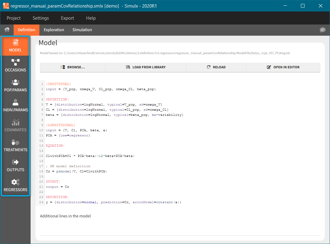
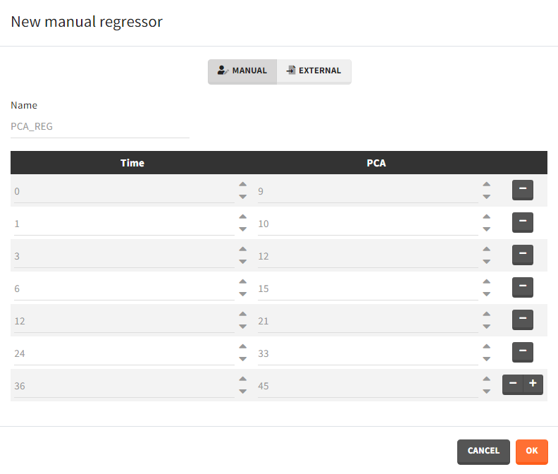
- Manual: It is a vector with manually defined time points and values, which are common for all individuals.
Example: parameter – covariate relationship with the covariate as a regressor
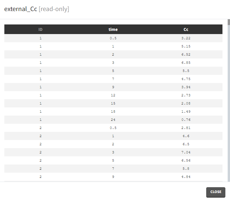
- External: Regressors definition is a table with the following mandatory columns: “time” for time points and “regressor_name” for regressor values. Optionally, it can have a column “id”. In the absence of the “id” column, the time grid is equal for all individuals and occasions (if defined in the model).
Example: PK-PD model with PK measurements as a regressor
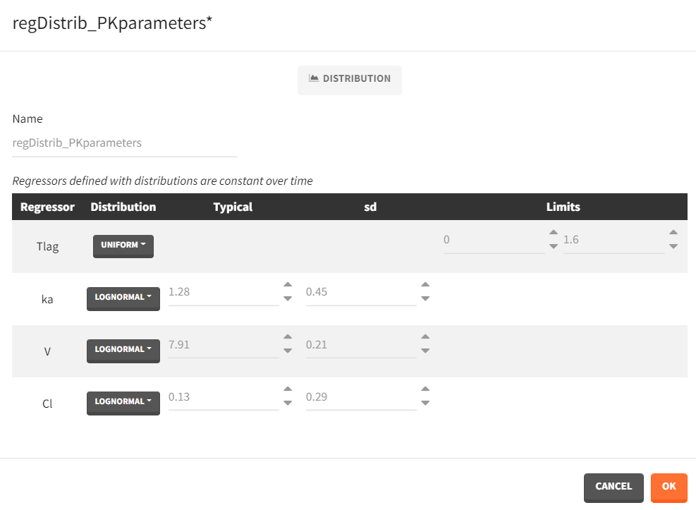
- Distribution: The regressors are described via distribution laws which define their value across individuals. When a distribution is used, the regressor is considered as constant over time. When used in the simulation, new regressor values are sampled from the defined distributions for each individual. The distribution for each regressor can be normal, lognormal or logitnormal with a mean and sd, or uniform with a lower and an upper and bound. If the distribution is lognormal or logitnormal, sd is the standard deviation of the distribution in the Gaussian space, i.e \(V_{reg}=V_{typical}\times exp(\eta)\) with \(\eta \sim N(0,sd^2)\). The typical value is the median of the distribution.
Defining a regressor element as a distribution is convenient for sequential PD model where individual PK parameters have been defined as regressors. After exporting the project to Simulx, new individual PK parameters can be sampled by defining the regressor element for the individual PK parameters as a distribution. Note that correlation terms are not possible.
Interpolation between defined values
Regressors are defined over time for a finite number of time points. In between those time points, the regressor value can be interpolated in two different ways:
- last value carried forward: if we have defined \(reg_A\) at time \(t_A\) and \(reg_B\) at time \(t_B\)
- for \(t\le t_A\), \(reg(t)=reg_A\) [first defined value is used]
- for \(t_A\le t<t_B\), \(reg(t)=reg_A\) [previous value is used]
- for \(t>t_B\), \(reg(t)=reg_B\) [previous value is used]
- linear interpolation:
- for \(t\le t_A\), \(reg(t)=reg_A\) [first defined value is used]
- for \(t_A\le t<t_B\), \(reg(t)=reg_A+(t-t_A)\frac{(reg_B-reg_A)}{(t_B-t_A)}\) [linear interpolation is used]
- for \(t>t_B\), \(reg(t)=reg_B\) [previous value is used]
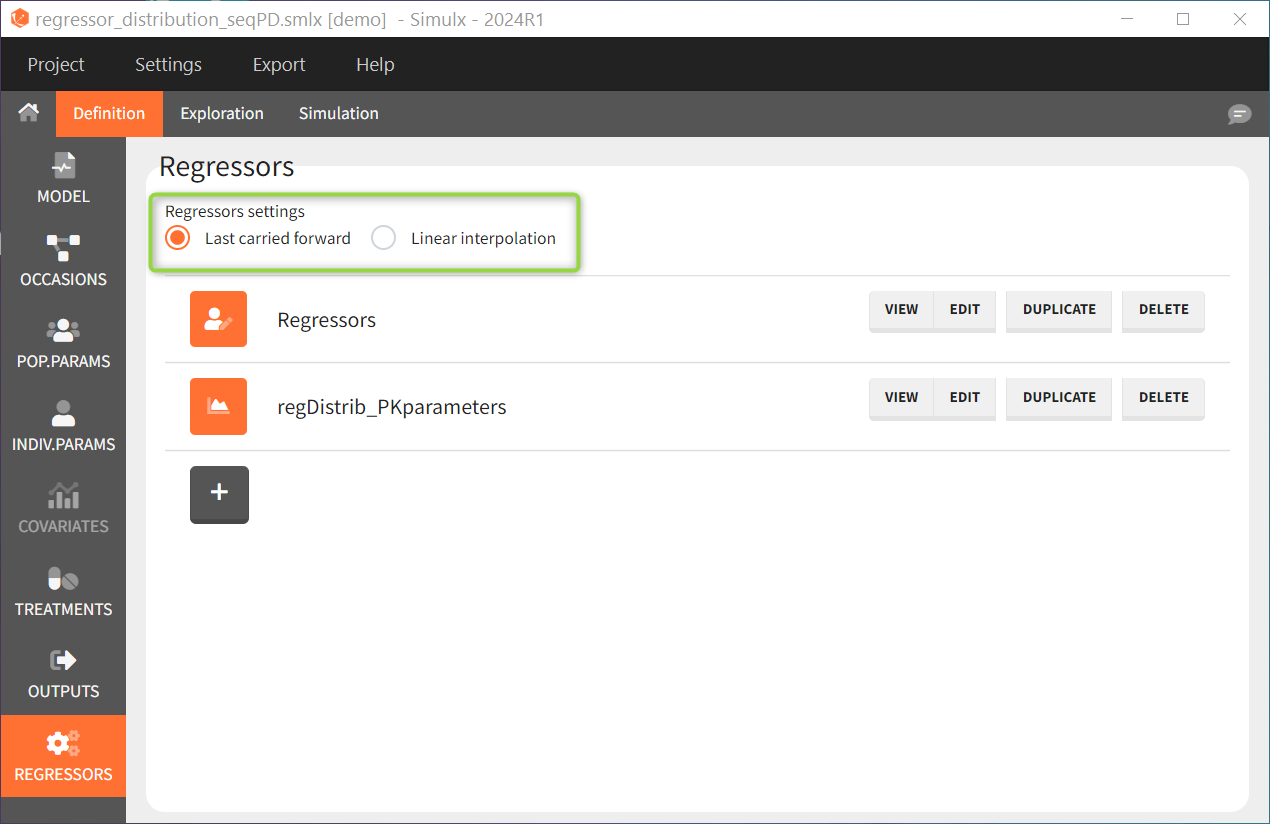
This can be chosen in the DEFINITION > REGRESSORS tab and applies to all defined regressor elements.
Regressors imported from Monolix
Importing a Monolix project generates automatically regressors element with regressors names from the dataset:
- mlx_Reg: contains Ids, times and regressors values read from the dataset. Occasions are included if any.
- mlx_RegDist: (created only if all regressors of each subject and each occasion are constant over time) element of type “distribution” with typical values, standard deviations and probabilities calculated on the individuals of the Monolix project. No correlation between the regressors is assumed. Regressors having only strictly positive values in the Monolix dataset are assumed to follow a log-normal distribution, and the others are set with a normal distribution.
3.Exploration
The Exploration tab is the second tab in the interface of Simulx. It simulates a typical individual to explore a model by interactively changing treatments and model parameters.
- Simulate a single individual
- Compare treatments using exploration groups
- Display any non-random model variable as prediction output
- Interactivity: impact of parameters and dosing regimen on the model dynamics
- Define new parameter or treatment elements
- Add observed data in the plot
- Select elements for Simulation of clinical trials
- Plots settings
- Export the plots as images
Predicted individual
In Exploration, the predictions are based on only:
- one set of individual parameters (mandatory),
- one or several treatments (optional) for one individual,
- one or several outputs (mandatory) with a single vector of measurement times per output,
- one set of regressor values, only if regressors are present in the model (mandatory).
These elements are selected in the left panel.
Thus an element of type “Individual parameters” must be selected, and it is not possible to select an element of type “Population parameters“.
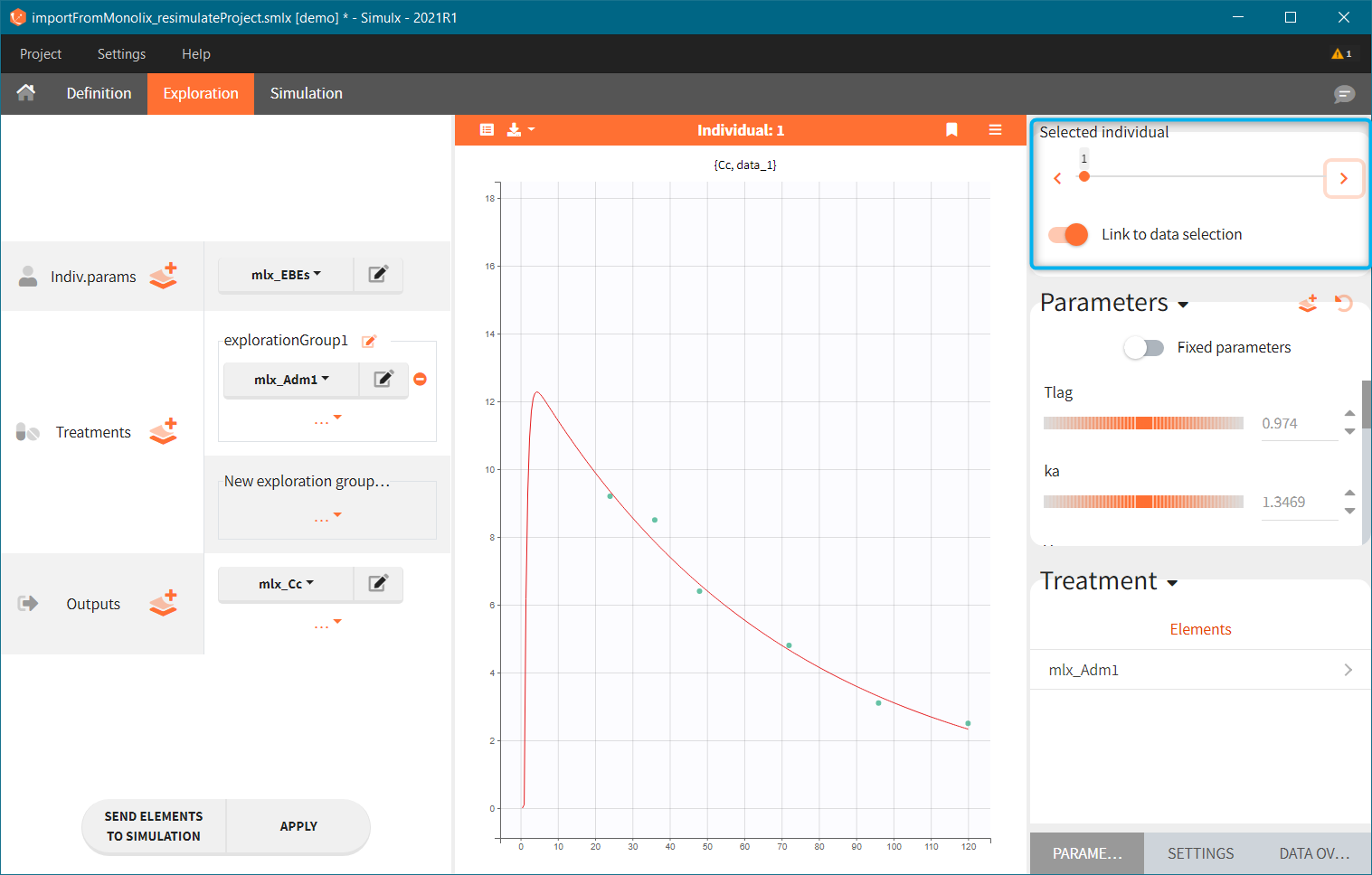
If a selected element is a table containing several sets of individual values, then the first row in the table is selected by default, and the “ID” field on top of the plot in the middle allows to select the row in the table corresponding to a particular ID.
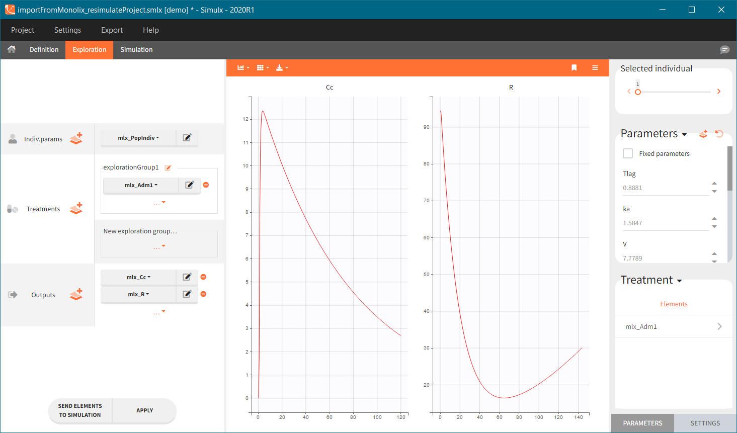
[Demo: 1.overview/importFromMonolix_resimulateProject.smlx]
This field is highlighted on the figure below, corresponding to a project that comes from a Monolix project imported into Simulx:
-
- the individual parameters come from the table mlx_EBEs contains the EBEs estimates,
- the treatment mlx_Adm1 contains the individual doses imported from the dataset used in Monolix,
- the output mlx_Cc contains a single vector of regular measurement times for Cc, the structural model output.
Thus changing the “ID” value will change the row read from the two tables mlx_EBEs and mlx_Adm1.
Exploration groups
- 3.exploration/PK_exploration.smlx
Treatment can contain several elements in different exploration groups (explorationGroup1 and explorationGroup2 below), or combined within an exploration group (as in the explorationGroup2 below). Each exploration group produces a separate prediction. If an exploration group contains several treatments, then the prediction corresponds to the treatments given together to the same individual.
In the demo shown below, there are two exploration groups: the first corresponds to the treatment element singleDose_150, while the second corresponds to the combination of loadingDose_100 and multipleDoses_50. Two prediction curves in different colors represent these two exploration groups in the plot.
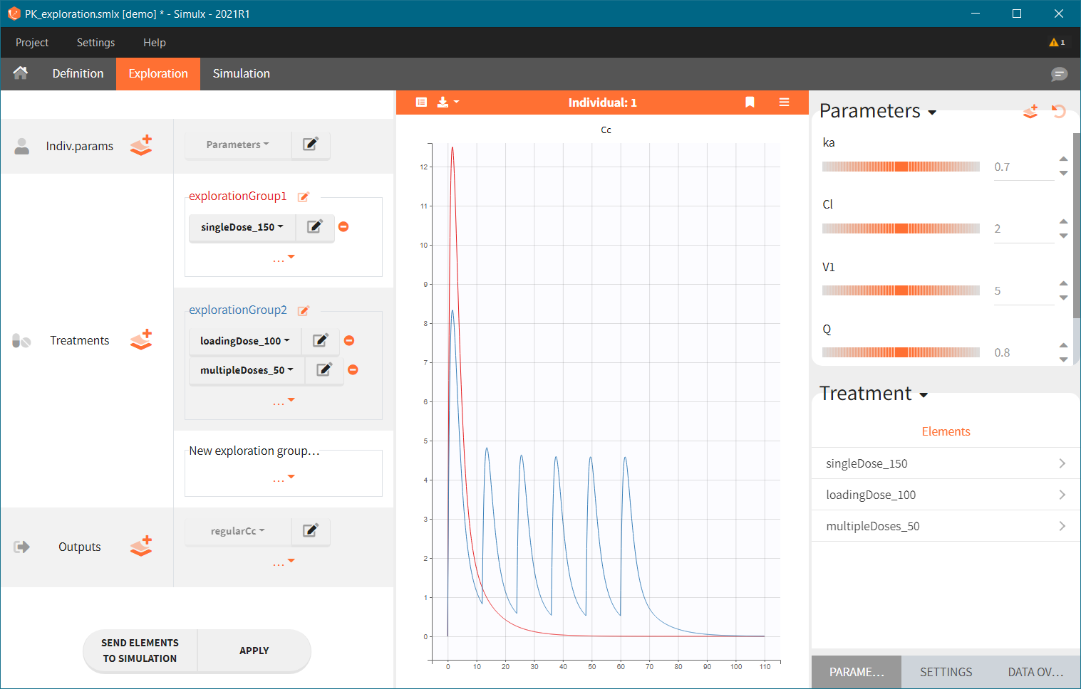
Exploration outputs
- 3.exploration/TMDD_exploration.smlx
Only non-random element of type “Output” can be selected in Exploration, thus they should:
-
- correspond to continuous variables (consequently excluding time-to-event, categorical or count variables)
- not include a residual error model in their definition.
By default, there is a separate plot for each selected output, as shown below. This can be changed in the exploration settings, where it is possible to select variables to display at each chart. If the scenario contains several output elements based on the same variable (but on a different grid), then they are plotted on the same plot with merged grids.
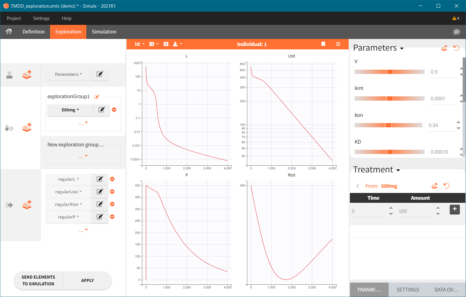
Interactive modification of parameter values or dosing regimen
- 3.exploration/PK_exploration.smlx
The right panel of the Exploration tab has three sub-tabs: PARAMETERS, SETTINGS and DATA OVERLAY. The parameter values and dosing regimens can be modified there to explore in real-time their impact on the model dynamics.
The figure below shows the PARAMETERS sub-tab with the model parameters (Parameters) and treatment parameters (Treatment) sections (highlighted in blue). The parameter values can be changed via the small arrows, sliders or by entering new values with the keyboard. The “reset” button ![]() resets parameters to their initial values, while the “new” button
resets parameters to their initial values, while the “new” button ![]() generates a new element (individual parameters element or treatment element) using the current values. On the plot, the solid curves correspond to the current predictions, while reference curves, added with the button
generates a new element (individual parameters element or treatment element) using the current values. On the plot, the solid curves correspond to the current predictions, while reference curves, added with the button ![]() , are shown as dashed lines.
, are shown as dashed lines.
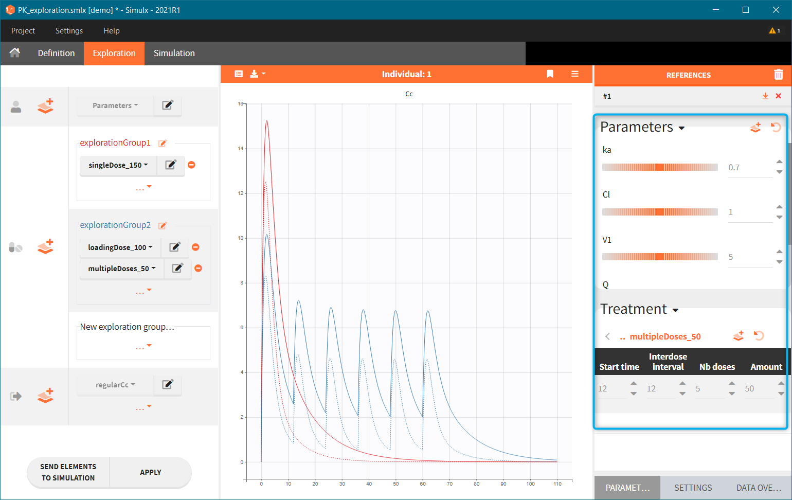
Reference curves. In the figure below, the section “Treatment” – highlighted in green – shows the elements from the treatment element: multipleDoses_50. All its parameters, such as start time, inter-dose interval, number of doses and dose amount can be modified. Current values can be set as a reference by clicking on the button ![]() – highlighted in purple. The reference curves are listed on the right panel – highlighter in blue – and are represented by dashed lines in the plot.
– highlighted in purple. The reference curves are listed on the right panel – highlighter in blue – and are represented by dashed lines in the plot.
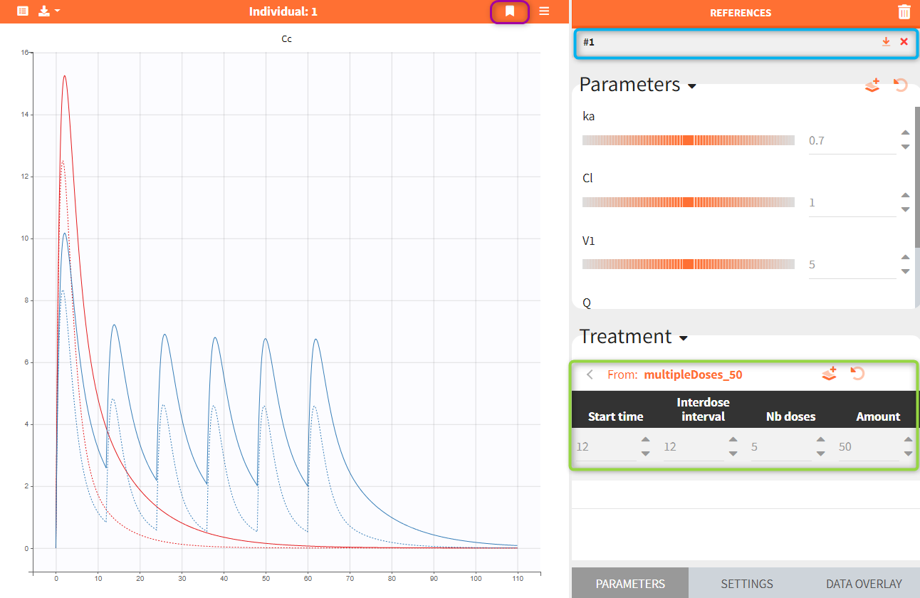
Several reference curves can be created and each successive one is displayed with a corresponding number. The icon ![]() restores the reference parameters values, and
restores the reference parameters values, and ![]() removes the reference curve from the list and from the plot. Hovering on a reference line (#1 in the figure below) highlights in yellow the corresponding reference curve, as seen in the figure below. Stroke dash-array defines the pattern of dashes and gaps of a curve.
removes the reference curve from the list and from the plot. Hovering on a reference line (#1 in the figure below) highlights in yellow the corresponding reference curve, as seen in the figure below. Stroke dash-array defines the pattern of dashes and gaps of a curve.
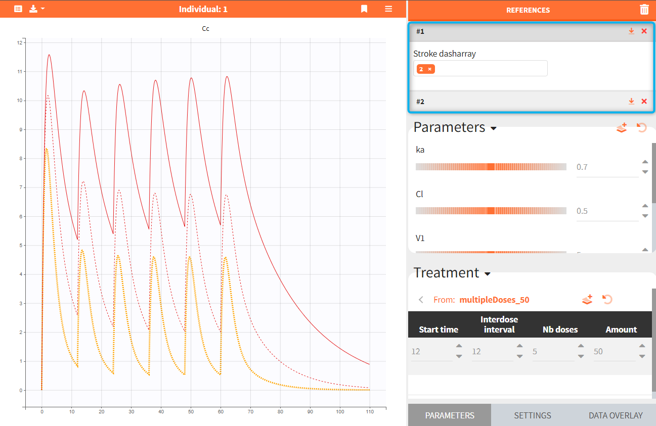
Defining new parameter or treatment elements
- 3.exploration/PK_exploration.smlx
Exploration allows to create new elements from the current values by clicking on the icon ![]() . In the parameter section it creates the Individual parameters element, while in the treatment section it creates the Treatment element.
. In the parameter section it creates the Individual parameters element, while in the treatment section it creates the Treatment element.
A window to define a new element opens automatically. For the parameters, the individual parameter element is of type “manual” and by default replaces the previously selected element in the Exploration scenario. Untick the corresponding checkbox (blue mark in the figure below) to only define a new element – without the replacement.
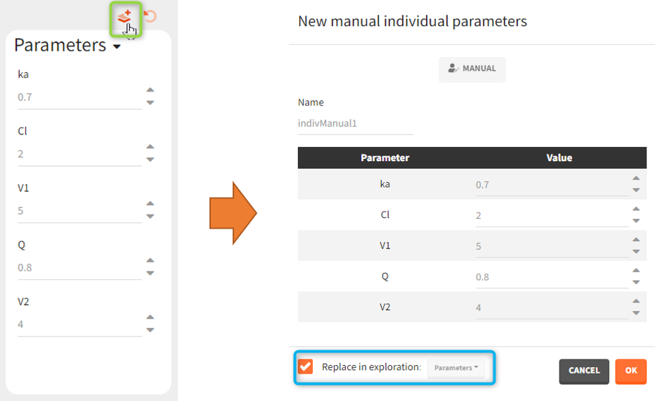
A new treatment element can be set as a regular or manual type – depending on the definition in the exploration. By default it replaces the treatment element used in the exploration, but it can be also added as the new treatment to a new exploration group.
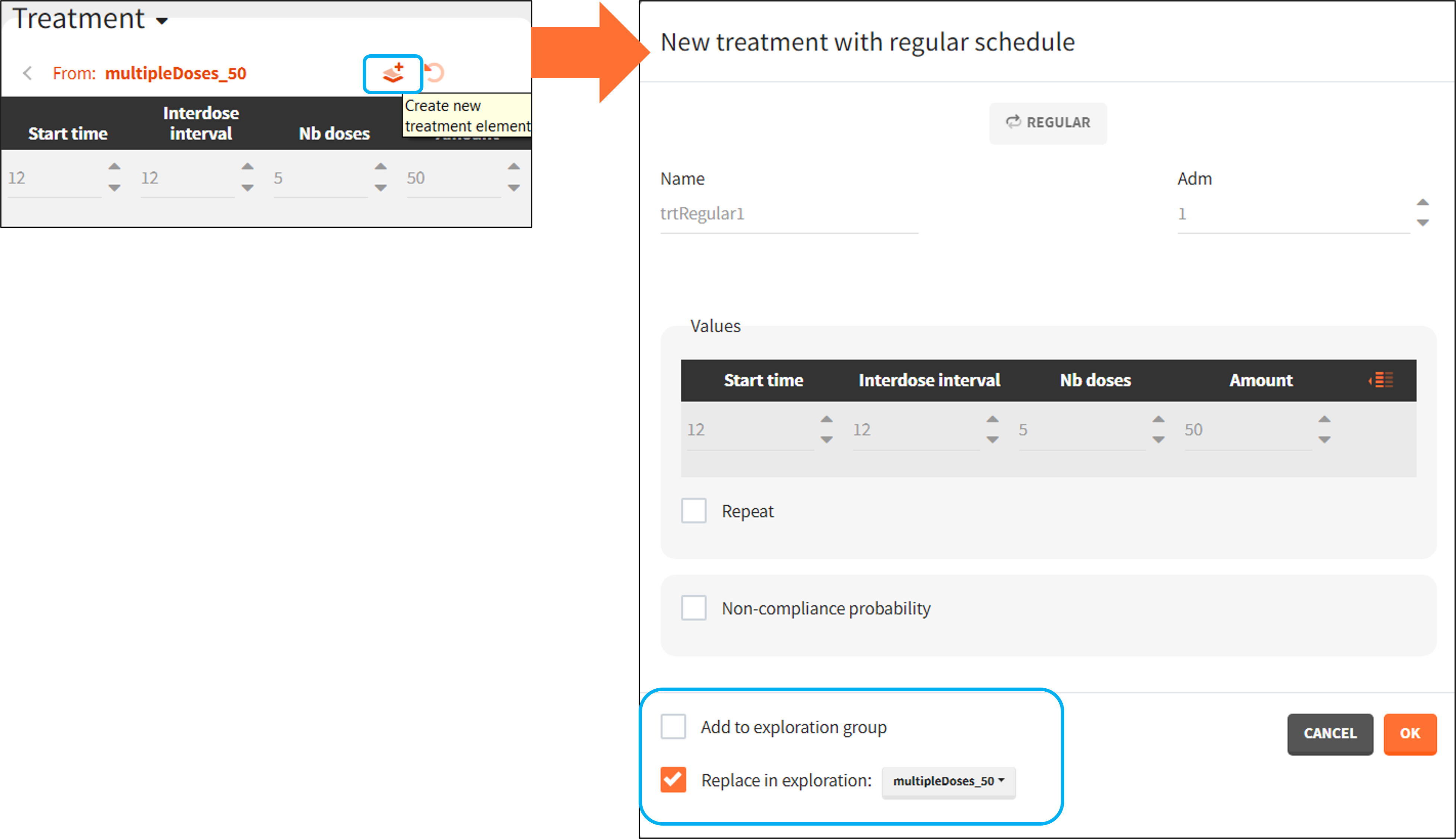
Overlay of the observed data
Continuous data can be overlaid on the prediction plots.
Load
Data overlay sub-tab in the Exploration tab allows to load a data file. Click on the BROWSE button and select a file. It has to be a Monolix compatible dataset and has to contain columns that correspond to: subject identifier (tag: ID), time of observations (tag: TIME) and observation values (tag: OBSERVATION). It is possible to have multiple observations to be displayed in different charts. In this case, the loaded datafile need to contain the column with observation id to distinguish different observations.
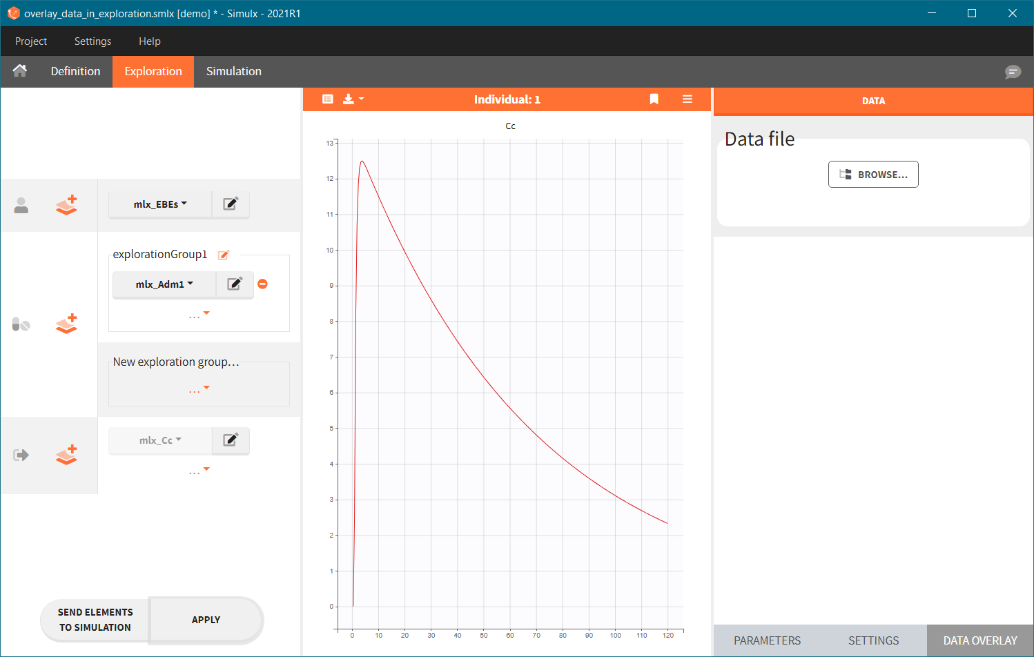 |
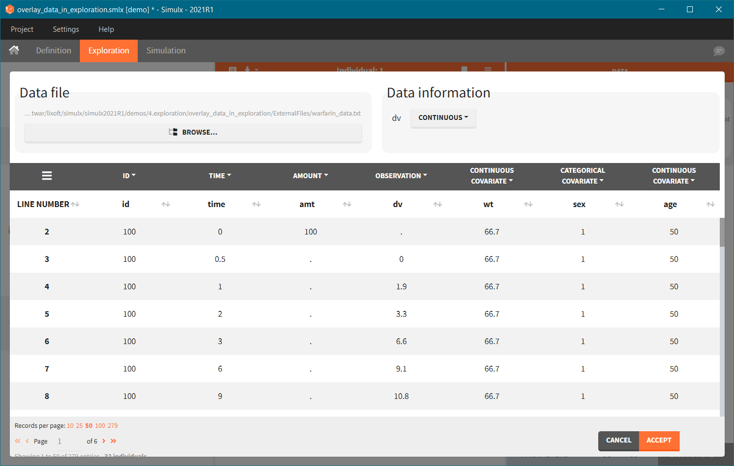 |
After tagging columns, click on the ACCEPT button to load the data file. Displayed observations can be filtered (green frame) using categorical covariates present and correctly tagged in the loaded file. In the figure below, ticked box next to a value “0” means that in the plot there are only observations for individuals with SEX = 0. To change the tagging, click on the VIEW/EDIT button (blue frame).
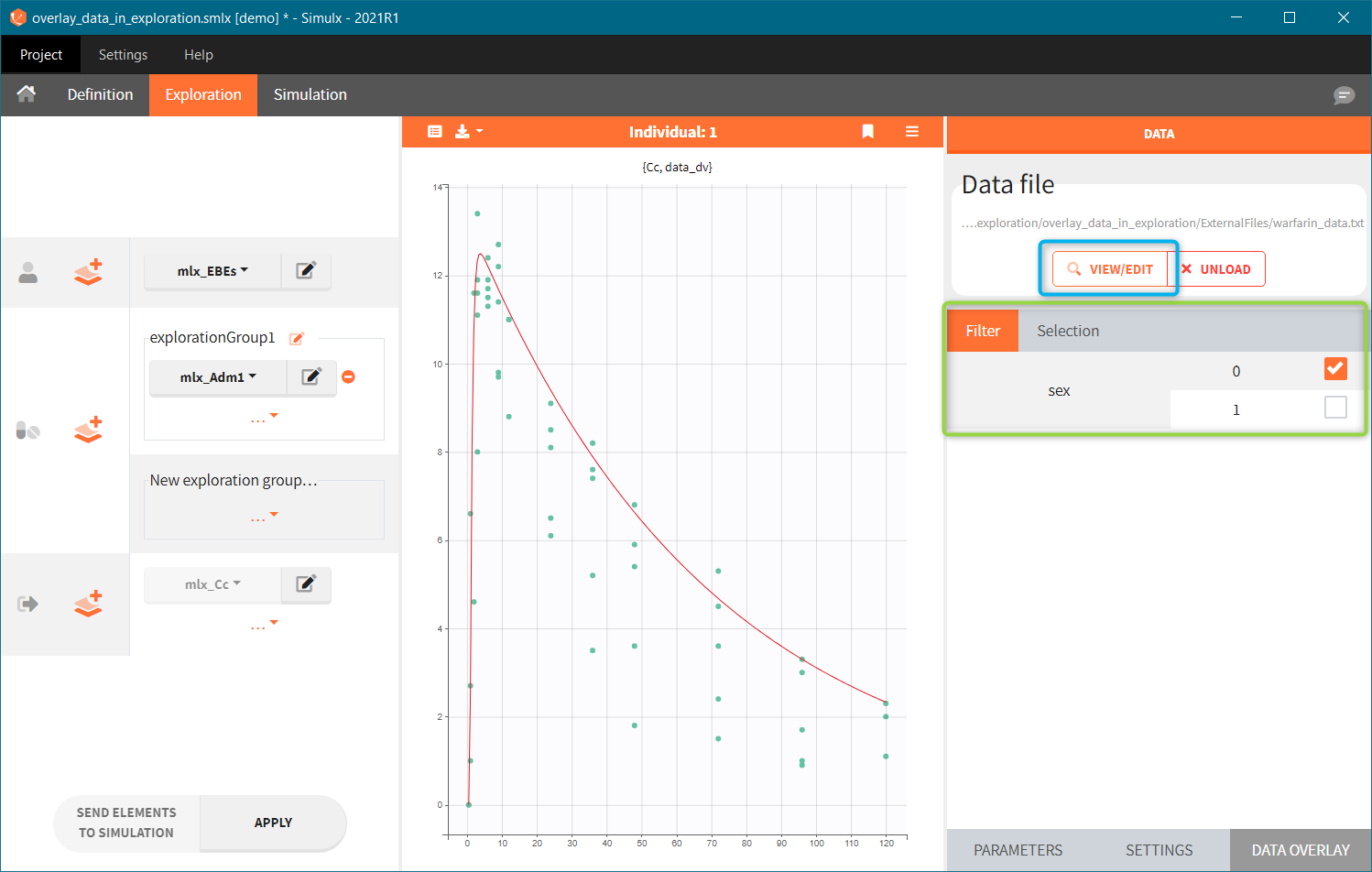
When a Simulx project is build by importing a Monolix project, then the dataset – used in the Monolix project – is set automatically in the DATA OVERLAY sub-tab.
Display
Observed data are displayed automatically as “dots” if there is only one output in the Exploration scenario and the data file contains only one observation type. Otherwise – in case of several different outputs or multiple observations types – data display has to be selected in the SETTINGS sub-tab.
In the data – charts grid, see the figure below, observation data are listed in rows. Numerical order is applied if the observation identifiers in the data file are integers, eg. data_1, data_2, …; or alphabetical order if the observation identifiers are strings, eg. data_PD, data_PD, as in the figure below. Charts are in columns. To display data on a chart, click on the drop-down menu of ![]() in the appropriate grid cell and select “dots” or “lines”.
in the appropriate grid cell and select “dots” or “lines”.
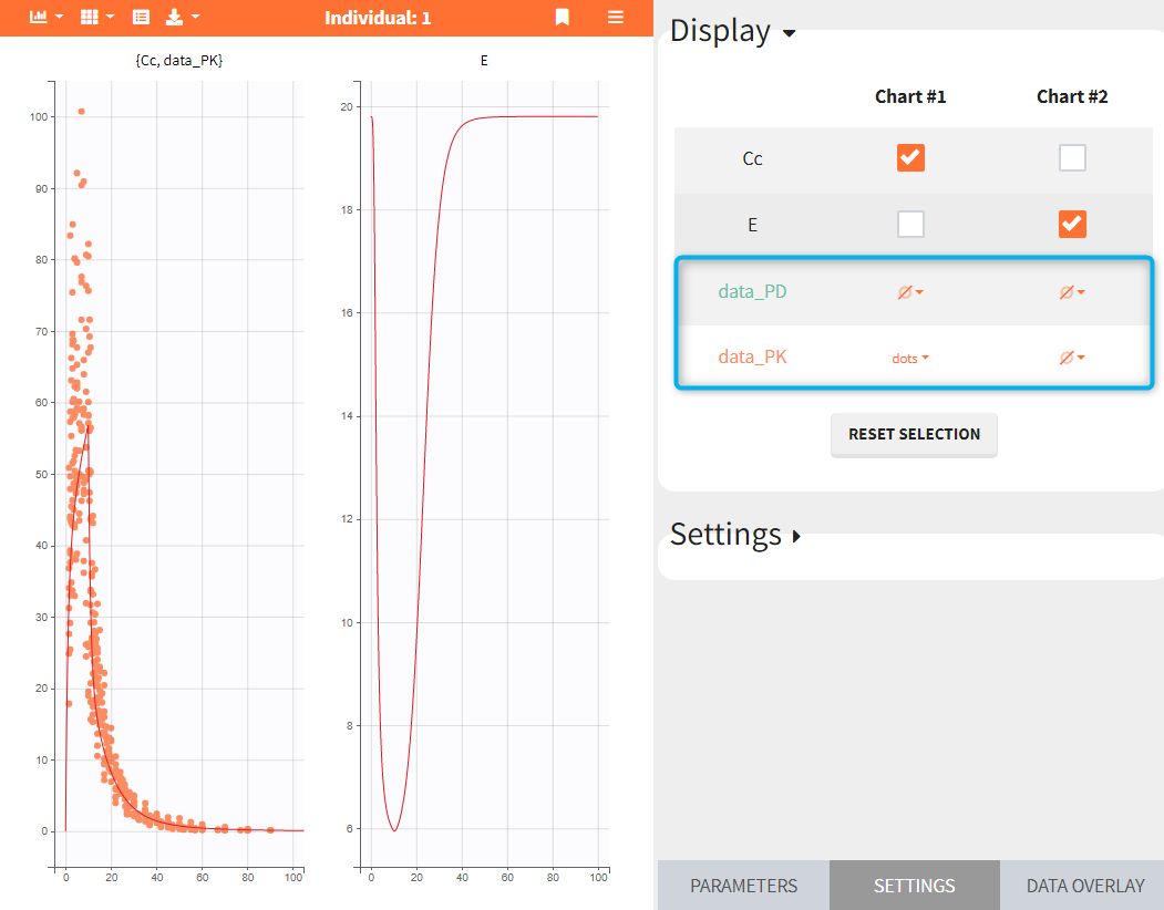
Link to individual selection
If any of the exploration scenario elements contains a table with several individuals, then the simulated individual can be selected in the PARAMETERS sub-tab, see individual prediction description section for details. To link the observed data to the selected individual, enable the toggle “Link to individual selection”. Only data corresponding to the selected individual will be displayed on charts. The option “Link to individual selection” only appears if the list of ids found in the data set and in the elements selected for the simulation are the same.
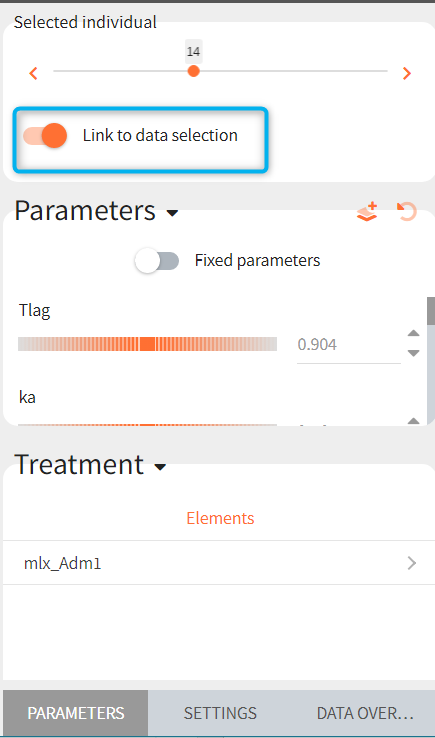
It is also possible to display one or several individuals selected from the dataset, which may or may not be linked to the simulated individual. This option is available in the DATA OVERLAY sub-tab, in the “Selection” section. In the example below, selection contains a range of IDs between 15 and 42 and only observed data corresponding to these individuals are overlaid on the chart.
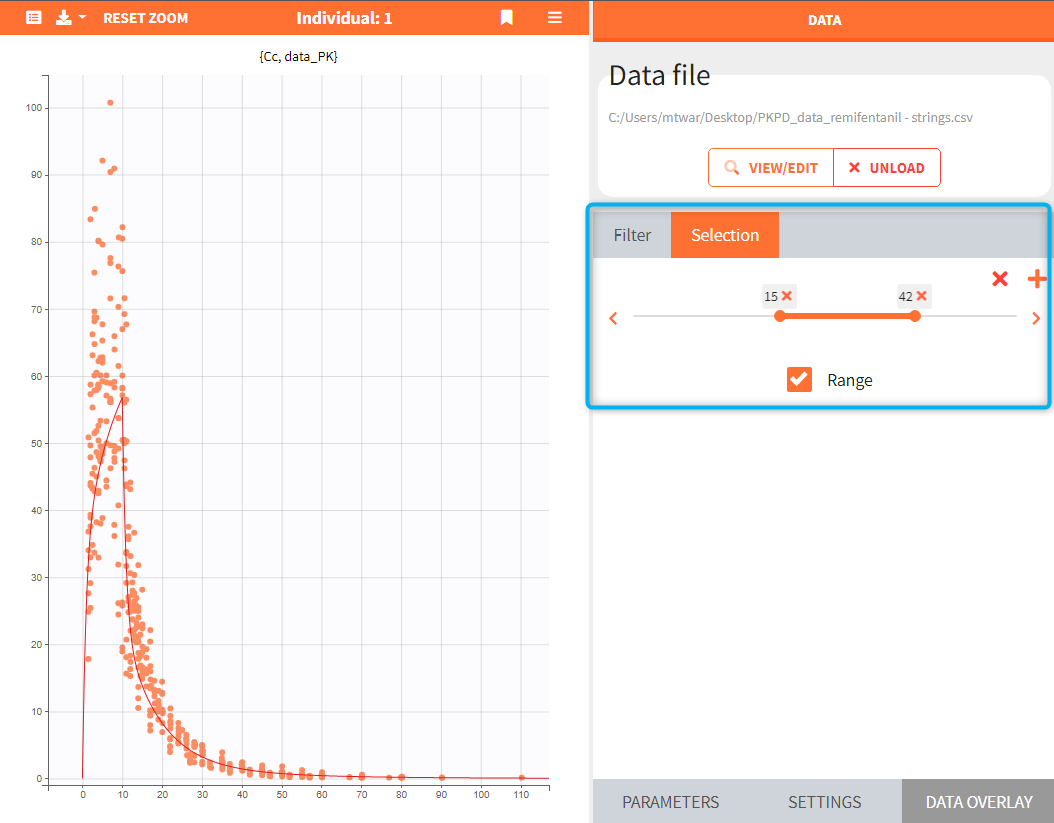
Sending elements to simulation
The button “Send elements to simulation” sends all elements selected in the Exploration to the scenario definition in the tab Simulation. Exploration groups are turned into simulation groups with a default size of 1 individual per group.
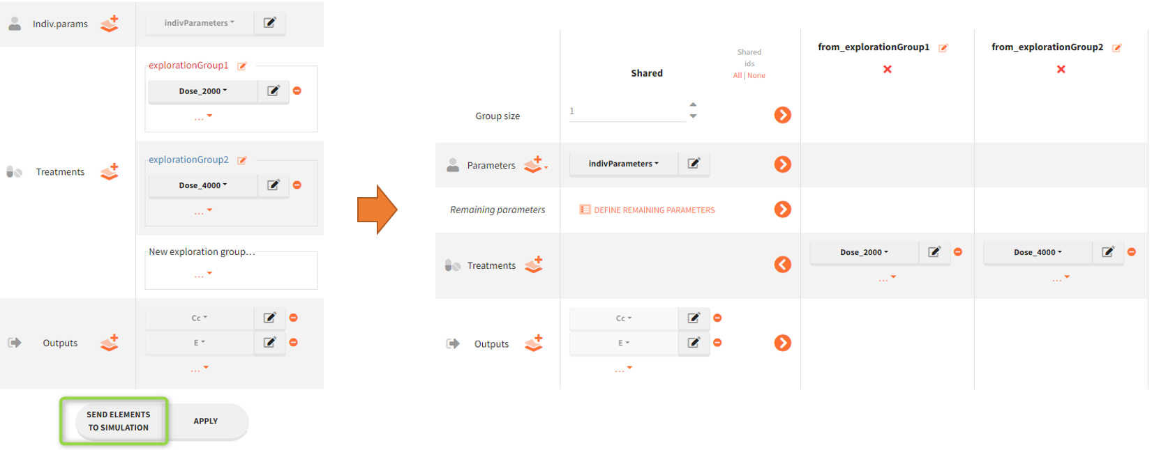
Plots settings
The panel “Settings” can be used to control plots features, such as the scale of the curves displayed on each plot and axis limits. The x-axis is common for all charts, while the y-axis can be specified independently for each chart.
In the following figure, two variables Cc and E are displayed on separate charts. They have the same x-axis limits – blue frame. The y-axis is specified for each chart: user limits 0-60 on the chart – 1, and automatic limits on the chart – 2 – green frame.
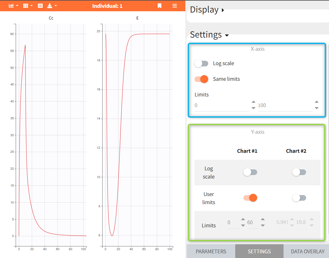
Exporting plots
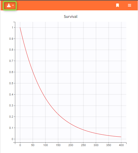
The “export” button on top of the plots can be used to save the plots as an image in the result folder. Two image formats are available: PNG and SVG (Scalable Vector Graphics).
4.Simulation
The main goal of Simulx is to perform simulations of clinical trials. In other words, it simulates a population of individuals, in one or several groups, using different scenarios. It gives the last step of the modeling&simulation workflow, after model building in Monolix for instance.
There are two tasks in the simulation tab: SIMULATION that generates outputs, and OUTCOMES & ENDPOINTS – a post-processing task – that uses the simulation outputs to calculate outcomes (one per individual) and endpoints (summary over all individuals of a group). In addition, running the tasks produces and immediate feedback thanks to the automatically generated RESULTS and PLOTS.
Simulations of clinical trials include:
- Simulation scenario – Building a simulation scenario takes place in the dedicated section “Simulation” and includes selecting simulation elements, creating groups for comparison and choosing sampling options.
- Outcomes and endpoints – Outcomes & Endpoints are below the “Simulations” section. Outcomes represent a post-processing of the simulation outputs for each individual. Endpoints summarize the outcome values over all individuals, for each simulation group and for each replicate. It is a separate task, so it does not require re-running the entire simulation after a modification.
- Results – Results are in a dedicated tab as copyable tables. They include individual and output values, outcome&endpoint analysis and statistical group comparison.
- Plots – All simulation outputs, defined outcomes and endpoints are displayed on separate plots as individual outputs and distributions. In addition, plot settings, stratification options and charts preferences are available at hand in the right panel of the interface.
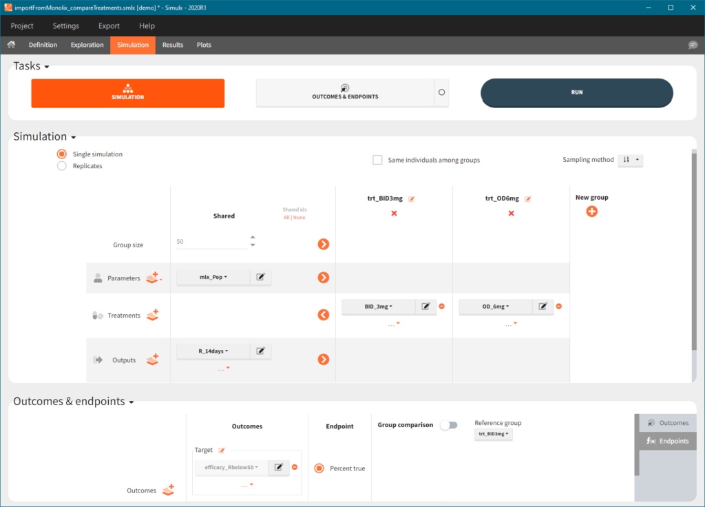
Order of events
There are prioritization rules in place in case of various event types occurring at the same time. So, the order of row numbers in the data set is not important, and same is true for the order of administration and empty/reset macros in model files.
The sequence of events will always be the following:
- regressors are updated,
- reset done by EVID=3 or EVID=4 is performed,
- dose is administered,
- empty/reset done by macros is performed,
- observation is made.
The behavior is consistent between Monolix and Simulx.
4.1.Building a simulation scenario
Simulx allows to interactively build a simulation scenario using simulation elements defined in the “Definition” tab and additional options available in the interface. It is done in the Simulations tab – Simulation section – which contains:
- List of simulation elements, which can be shared between groups or set as group specific.
- Flexible group definition with drop-down menus for selecting group specific elements and with editable group names.
- Option to run a single simulation or replicates.
- Different sampling options such as using subjects with the same individual parameters or drawing individuals from table type elements with different methods.
To run a scenario, just click on the button SIMULATION in the tasks section. When importing a Monolix project, Simulx automatically sets the scenario re-simulating the Monolix project.
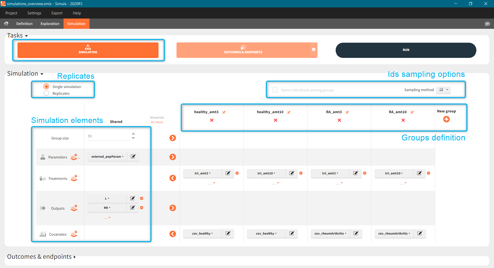
- Simulation elements
- Groups
- Replicates
- Sampling options and use of ids
- Sampling options
- Shared ids
- Same individuals among groups
Simulation scenario elements
List of simulation elements contains: group size, parameters, treatments, outputs and, if used in a model, covariates and regressors. To select an element from already defined elements, use a drop-down menu available after clicking on the currently selected element. To edit a selected element, click on the icon ![]() . To create a new element, click on the “plus” icon
. To create a new element, click on the “plus” icon ![]() to open a “New element” pop-up window in the Definition tab.
to open a “New element” pop-up window in the Definition tab.
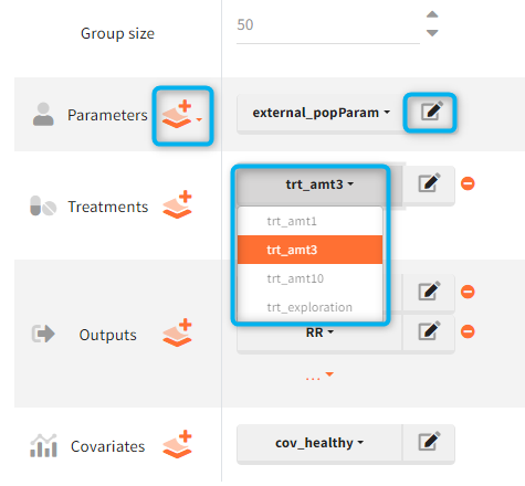
Mandatory elements
- Group size corresponds to the number of individuals in a group.
- Parameters can be chosen from POP. PARAM. or INDIV. PARAM. elements in the Definition. When Individual parameters are selected, then the covariate element disappears and new section to set the error model parameters becomes available.
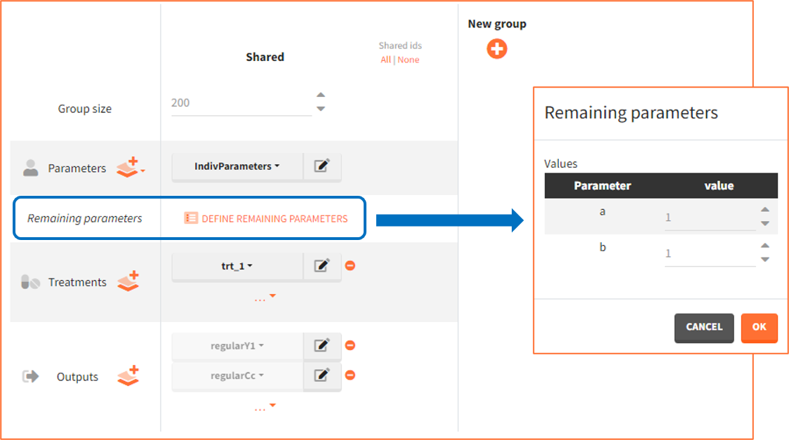
Note: Remaining parameters are all parameters that appear in the structural model (in the input line of [LONGITUDINAL]) and are neither individual parameters not regressors. They are typically error model parameters. These error model parameters will impact the simulation only if a noisy observation (from the DEFINITION section of the [LONGITUDINAL] block) is set as output element (instead of a smooth prediction in OUTPUT or variable in EQUATION).
- Outputs correspond to one or more variables to be computed and displayed in plots and results. When importing a project from Monolix, by default all observation outputs (if defined in a model) are automatically selected, otherwise only the last defined model output.
- Covariates are available in two situations: selected treatments use a covariate scaling or individual parameters model uses covariates and population parameters are selected as an element in the Parameters.
- Regressor is available only if it is used is a model.
Optional elements
- Treatment can be one element or a combination of several treatment elements.
- Occasions are optional even if defined in a model, but are mandatory if any occasion-dependent element is selected in a scenario.
Simulx automatically assigns default elements: the last one from the definition list of each category or specific default “mlx_” types after importing a Monolix, see here for details. It is not possible to remove in the Definition tab an element currently used in a simulation. However, it might not be possible to run a simulation if any of the mandatory elements was removes. For instance, deleting occasions element removes automatically all occasion-dependent elements even if used in a simulation.
Simulation scenario with groups
Groups allows to build a scenario with population having different characteristics, such as parameters, regressors, covariates, different treatments and/or different simulation outputs. Moreover, groups can have different number of individuals to compare clinical trial of different sizes.
To create a new group click on the “plus” button, use the arrows to move elements from “shared” part to group section (or vice versa) and select specific element for each group. Each simulation element can be shared between groups or can be a group specific.
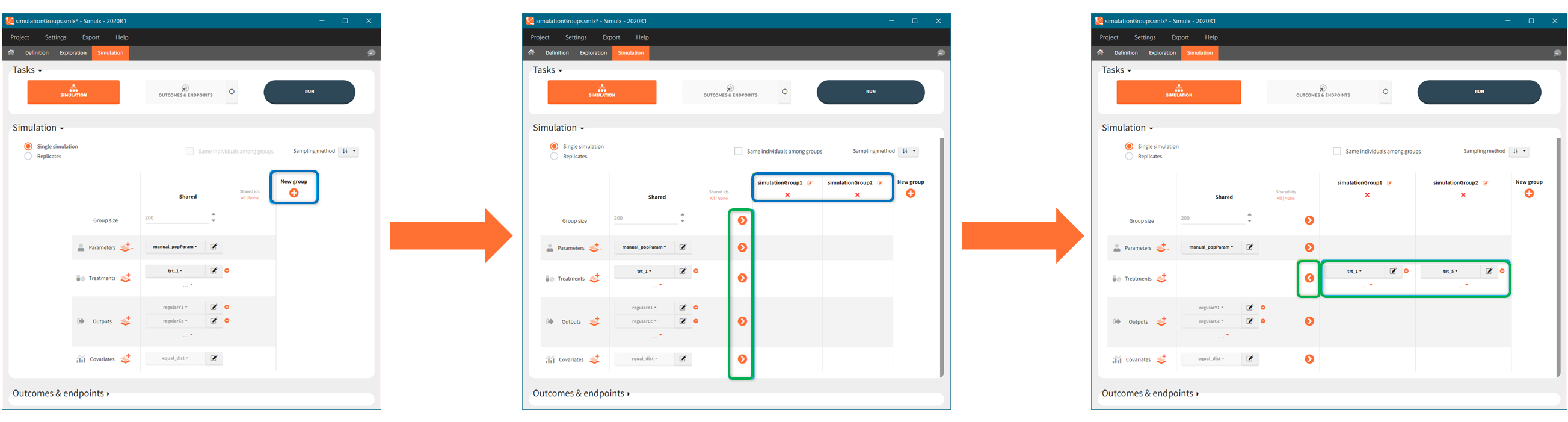
To edit a group name click ![]() next to it. In the Plots tab, figures for different groups appear in the same order as they are defined in the Simulation tab, not in the alphabetical order. To remove a group click “x” under the group name.
next to it. In the Plots tab, figures for different groups appear in the same order as they are defined in the Simulation tab, not in the alphabetical order. To remove a group click “x” under the group name.
- Each new group is by default a copy of the previous one (eg. group 3 is a copy of group 2).
- Population and individual parameters can not be used in different groups simultaneously.
Examples:
- [Demo 5.simulation: simulationGroups_treatment]: Simulation of three groups with three different oral dose levels: low (trt_1), medium (trt_5) and high dose (trt_10). Groups sizes, parameters, covariates and outputs are shared (the same) between the groups, while treatment is group specific.
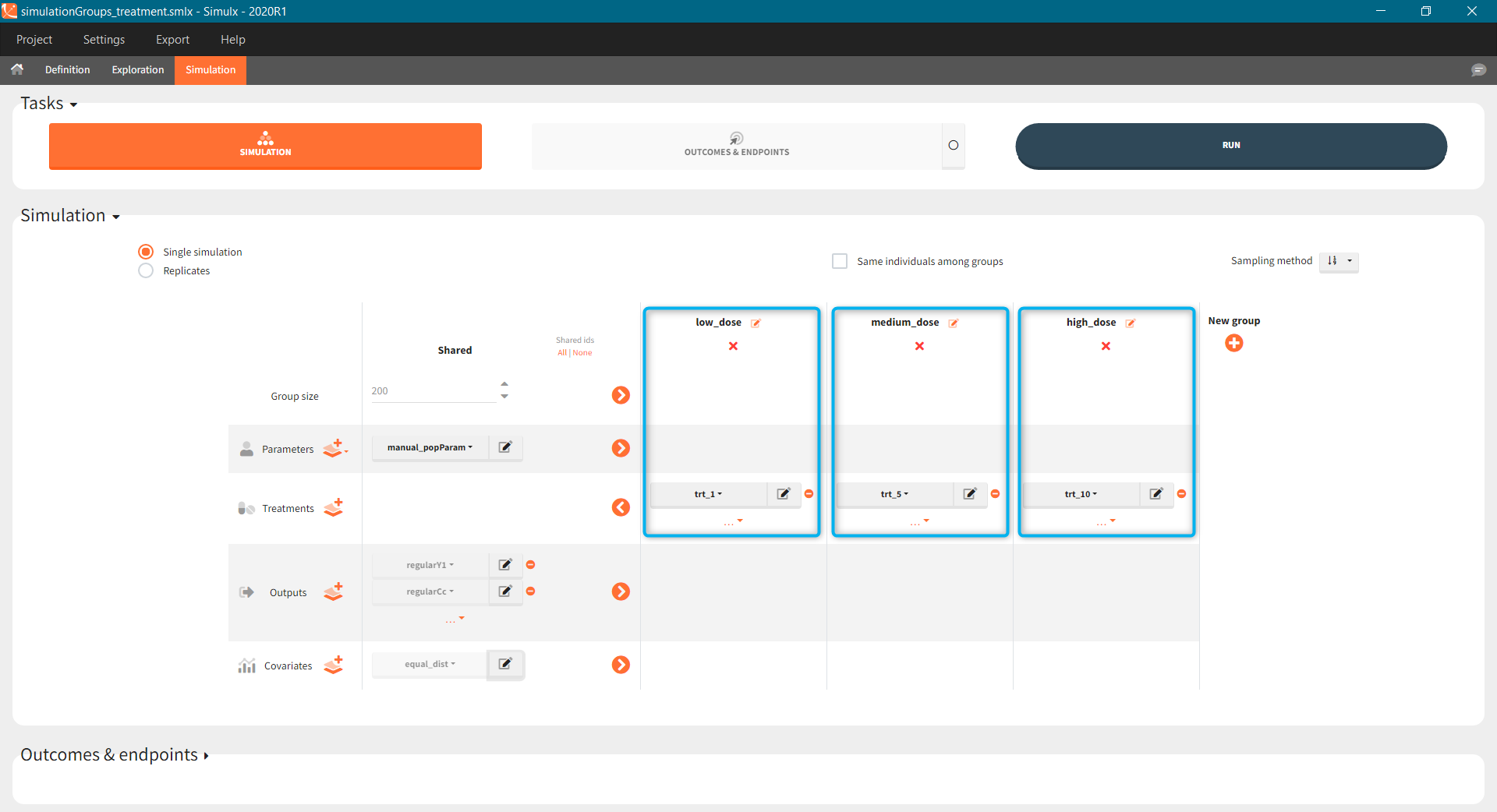
- [Demo 5.simulation: simulationGroups_ethnicGroups]: Simulation of two groups with different ethnicity, which affects the bioavailability. In this case, “covariates” simulation element is group specific with: “caucasian” modality for the first group and “asian” for the second group.
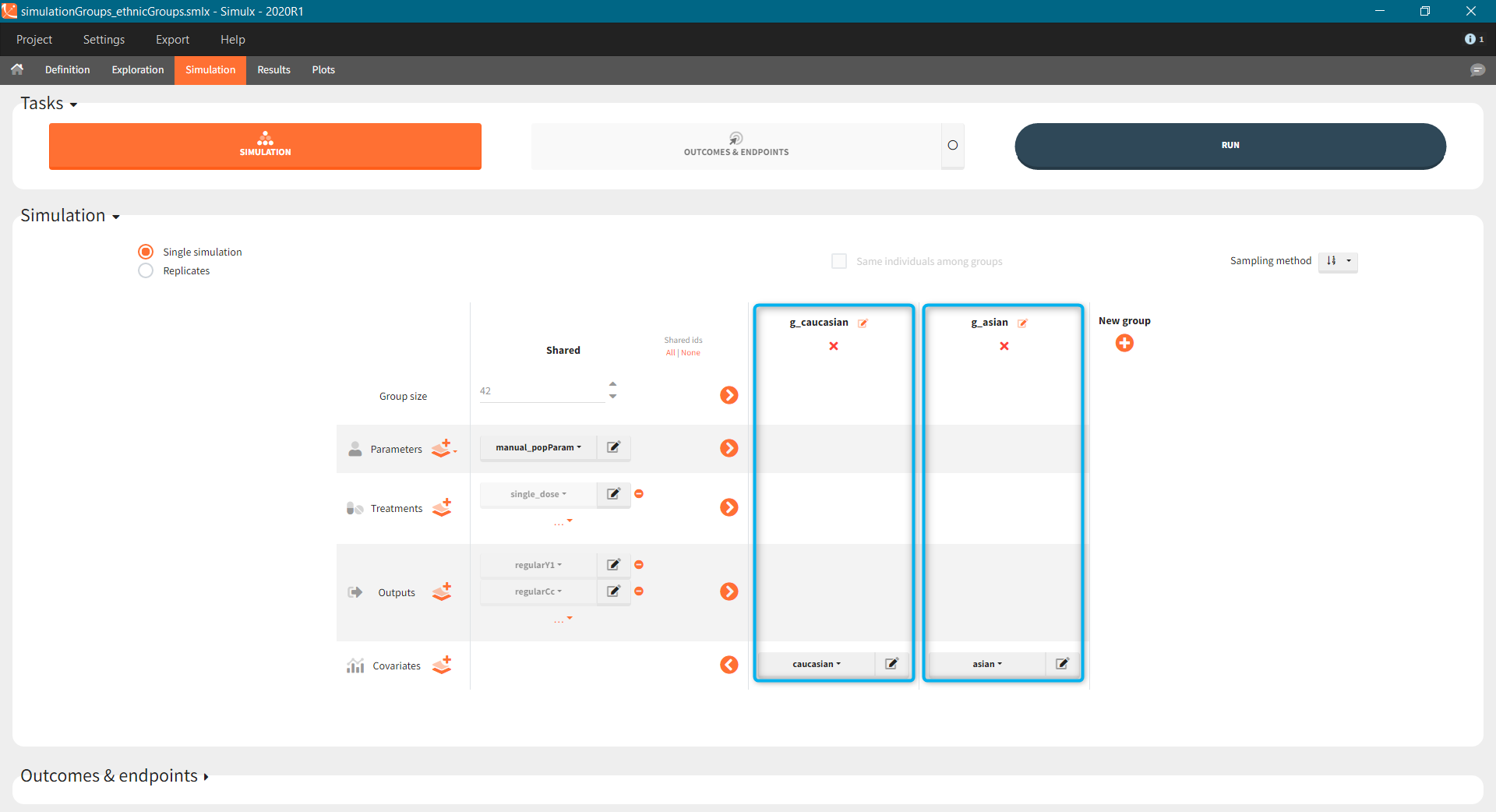
Simulation scenario with replicates
By default, Simulx simulates one clinical trial. When the option “replicates” is selected, then Simulx simulate the scenario several times.
- If population parameters are vectors (user-defined or imported from a Monolix project), then all replicates have the same population parameters.
- If population parameters are of a distribution type, then Simulx samples one set of population parameters for each replicate.
- If population parameters are given as an external table with several population parameters sets, for instance from the simpopmlx function, then each replicate uses one set of population parameters with the order of the appearance in the table.
Tables in the results tab display information for all replicates.
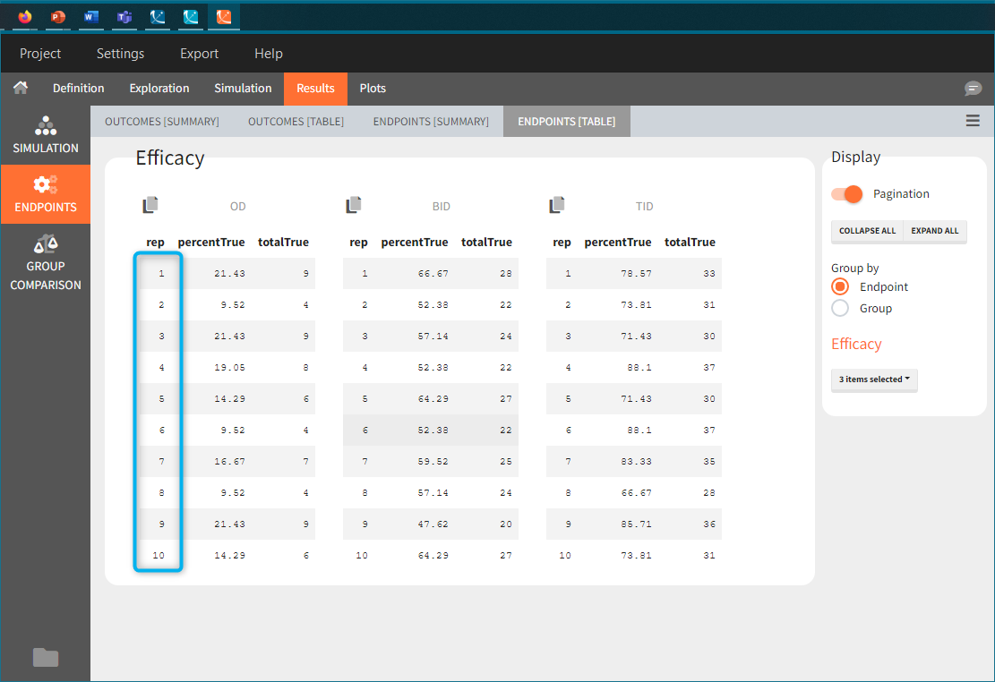
In “summaries” the values are summarized over all individuals and all replicates. For instance, endpoints result summarize outcomes over all replicates with the uncertainty of the result.
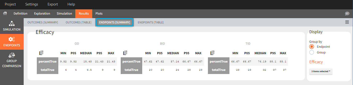
Similarly, plots contain information of all replicates. By default, individual outputs display only one replicate, however, stratification panel allows to select one or more replicate to plot (green frame).
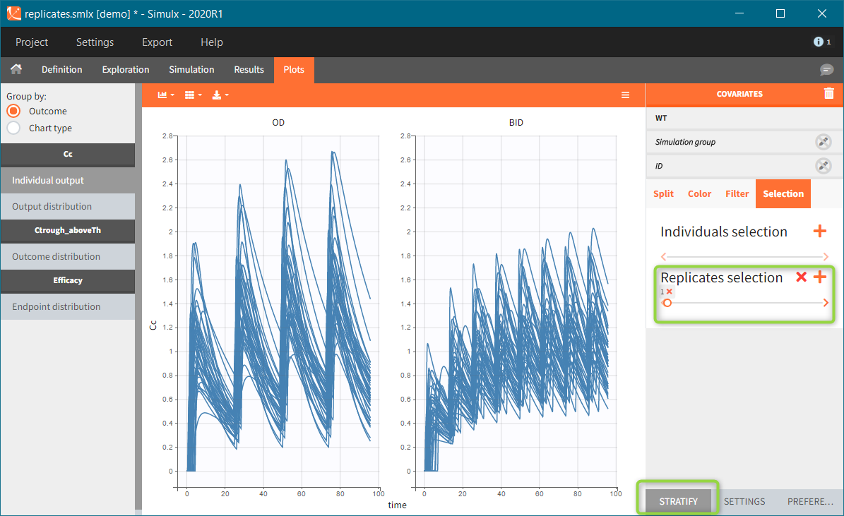
Endpoint distribution in case of replicates is summarized in a box plot.
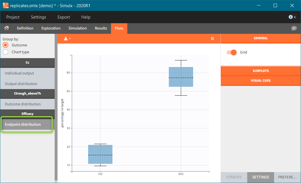
Sampling options
Individual sampling
Simulation elements of different types are subject to different individual sampling in a simulation. Elements defined as vectors provide common values for all individuals, so there is no sampling. When an element is a distribution, then sampling is done for each individual separately. Tables, from external files or from Monolix after importing a project from Monolix, can contain data for more then one individual distinguished with the column called “id”. In this case, there are three sampling methods available in the Simulation tab.
- Keep order (default) – individual values are taken in the same order as they appear in a table.
- With replacement – individual values are samples from a table with replacement.
- Without replacement – individual values are samples from a table without replacement. This option is available only if tables contain at least the same number of individual values as a group size.
All of the above sampling methods are general and apply to all tables in a simulation scenario.
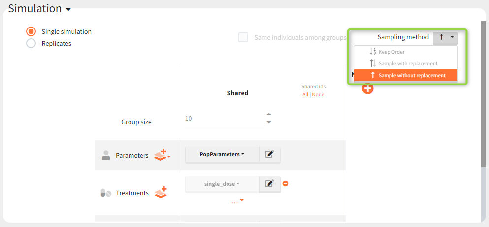
Shared ids
If there is a group of tables with individual values, an option “shared ids” allows to create an intersections of ids present in the considered tables. After that, ids from these intersection are sampled to create the data for simulation.
Example: Simulation uses a treatment with a dose amount depending on the patients weights. Treatment element and weights are external tables with columns (id, time, amount) for the treatment, and (id, weight) for the covariate. Moreover, an effect of the weight is added on the definition of the individual parameter (volume of the central compartment) in the model. It this case, it is important to match a sample from the treatment element with a sample from the covariate element. It is done by ticking two boxes in the “shared ids” column for both elements (blue frame).
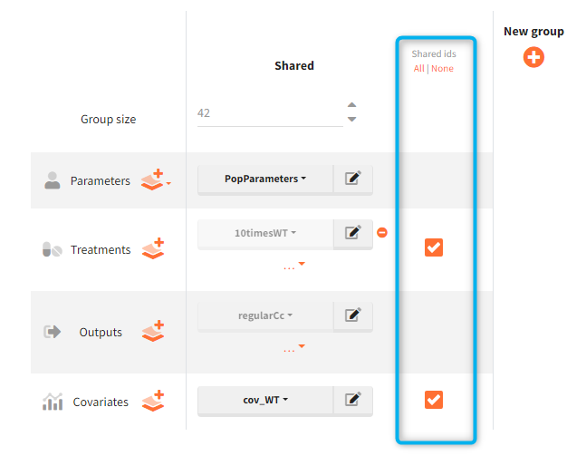
Same individuals among groups
“Same individuals among groups” option allows to have the same individual parameters in all groups and is available if the following elements (required for the sampling) are the same for all groups: size of groups, parameters (population or individual) and covariates. The main aim is to make the comparison between groups easier. In particular, it is used to compare different treatments on the same individuals – subjects with the same individual parameters. Selecting same individuals among groups assures that the differences between groups are only due to the treatment itself. To obtain the same conclusion without this option enabled, simulation should be performed on a very large number of individuals to averaged out the individual differences.
Example: a simulation of two treatment groups with shared parameters, covariates and outputs. When the option “same individuals among groups” is enabled, then subjects in each group have the same individual parameters because the same Parameters (manual_popParam) and Covariates (race) are used in all groups (Demo 5.simulation: simulationGroups_sameIdsInGroups).
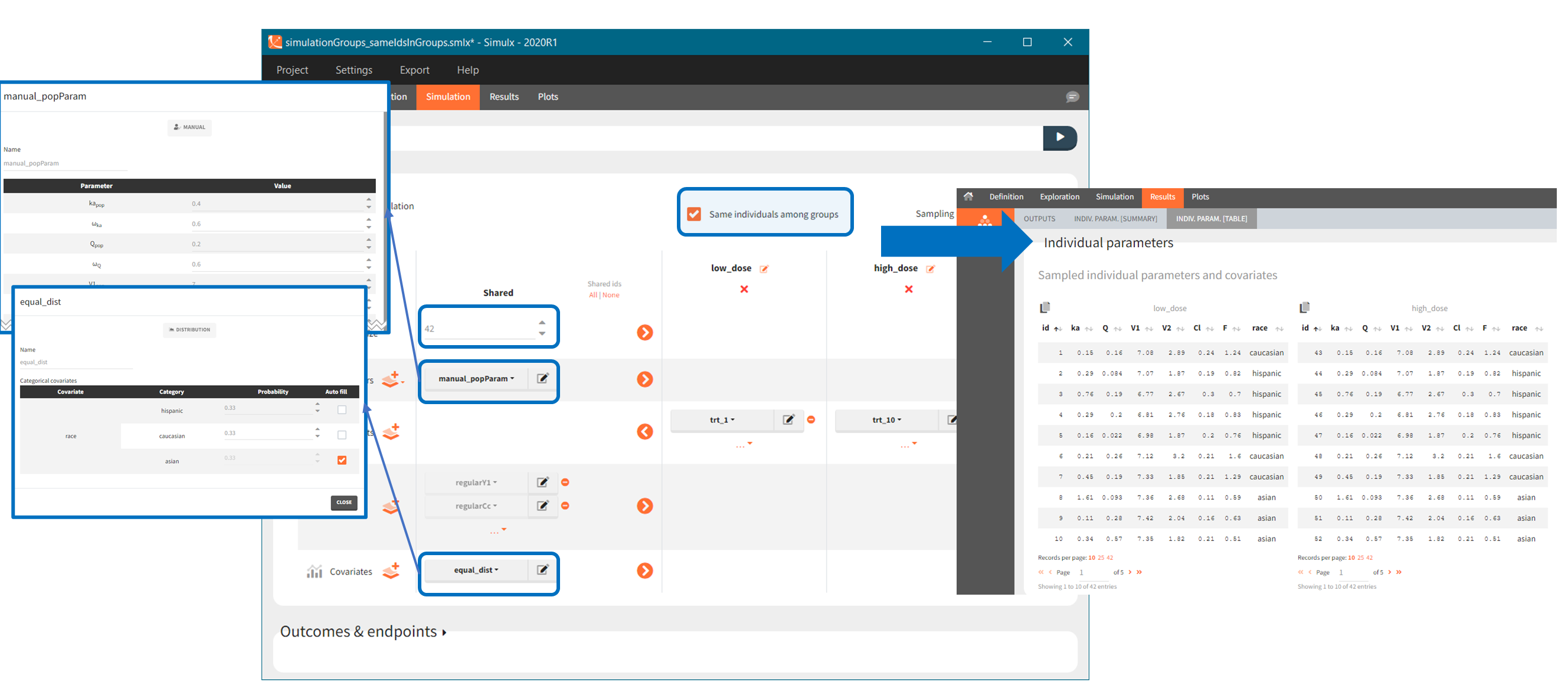
4.2.Outcomes and endpoints
Outcomes, endpoints group comparison are in a dedicated section “Outcomes&endpoints” of the Simulation tab.
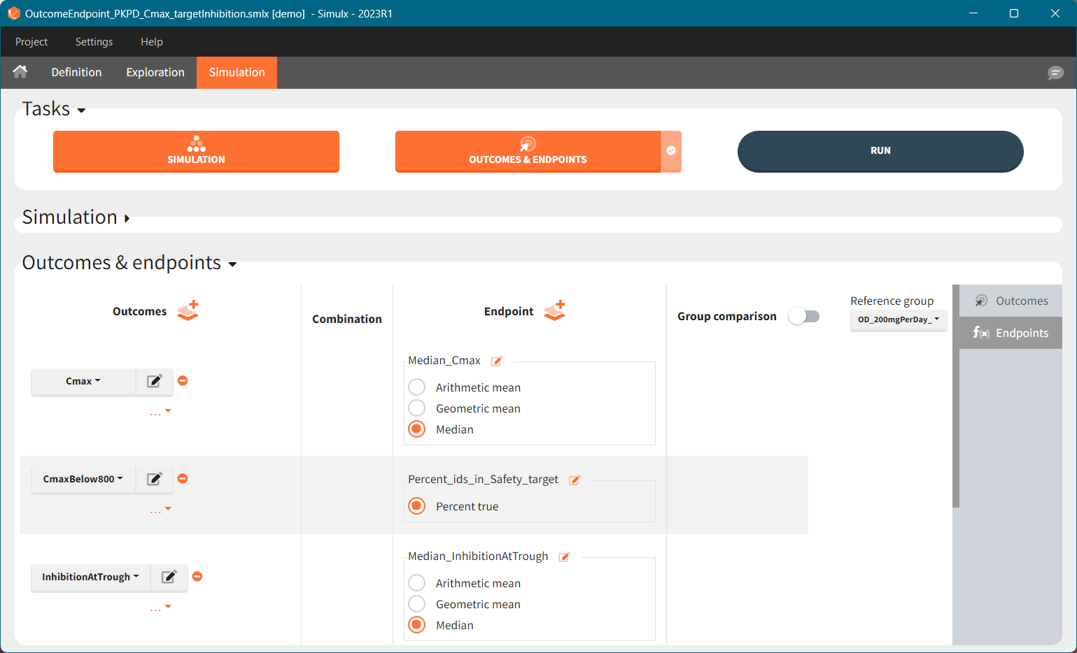
To calculate outcomes and endpoints click on the “Outcomes&Endpoints” button in the Tasks section (on top). The outcomes are a post-processing of the simulation outputs, so remember that you have to first run the “Simulation” task. You can also selected the task “Outcomes&Endpoints” in a scenario (circle radio button on the right hand side of the task button) and click the button RUN – Simulx will run both tasks automatically one by one.
The calculated values are displayed in the Results tab and Plots tab.
Outcomes
Outcomes represent a post-processing of the simulation outputs done for each individual. They correspond to the measure of interest per individual. Outcomes have different types: values (e.g Cmax), binary true/false (e.g true if Cmax < threshold), or time-to-event (e.g time to NADIR).
To create a new outcome, click on the “plus” button next to Outcomes header or on the “+ New outcome element” within the list of outcomes for an endpoint:
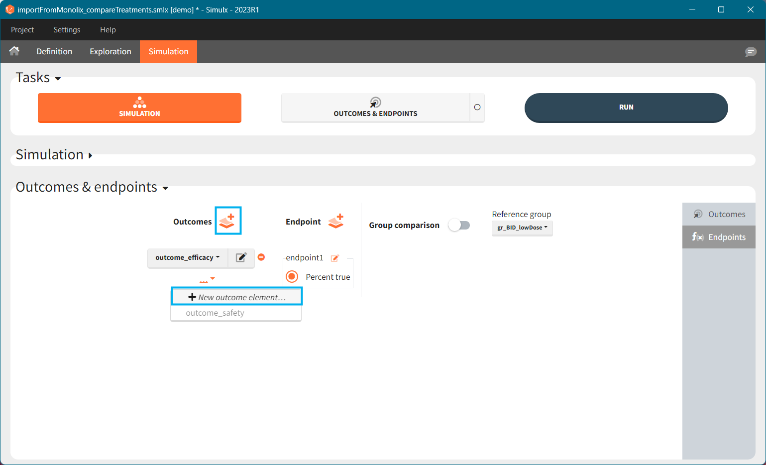
Each outcome has a name (default or user defined), which allows to select it in an endpoint definition. To define an outcome you have to select an output element for post – processing. You can only use output elements selected in the Simulation scenario. The specification of the outcome includes the following options to post-process the selected output.
For continuous, count and categorical outputs:
Relative to: none/ baseline/ maximal or minimal value/ maximal or minimal value up to current time/ custom value: it divides (“ratio”) or subtracts (“difference”) the output values by the specific value (i.e baseline – the first value of the output). For baseline option, because the first value of the transformed output is non-informative (ratio=1 or difference=0), it is removed.
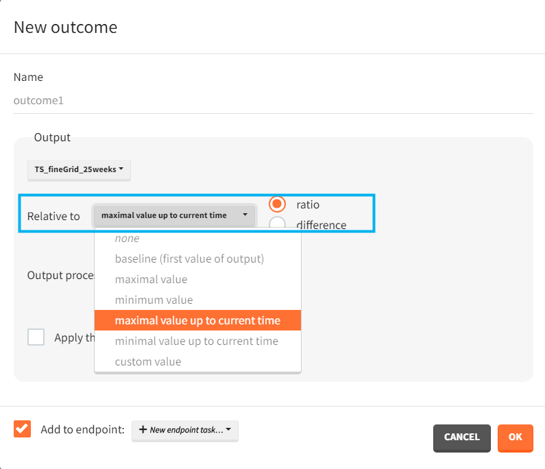
Output processing:
- average value – takes the average over all output values for each individual
- first or last value – takes a value at the first or last time point for each individual
- min or max value – takes the minimum or maximum over all output values for each individual. You can choose “value of min/max” to take the value of the min or max, or choose “time of min/max” to take the time of the min or max – as continues time or time-to-event.
- at custom point – takes a value of an output at a specified time point. Only grid time points are allowed.
- duration below or above a value or between values – calculates time when the output values are below, above or between a given values. Strict inequalities (< or >) apply. You input threshold values manually below the output processing menu. As duration you can choose:
- “cumulative time” – sum of time intervals between consecutive time points where output values satisfy the condition
- “% of total time” – cumulative time divided by the final time (in percentage)
- “number of observations” – number of time points where output values satisfy the condition
- “time of the first occurrence” – a time point where the condition is satisfied for the first time (can be event or continuous)
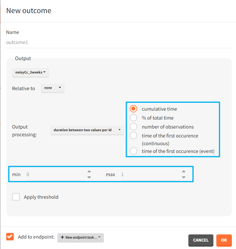
Apply threshold: applies a logical test (usually comparing the outcome value to a threshold) to get a binary true/false outcome. You must set a threshold value and a comparison sign (=, !=, >=, <=, >, <).
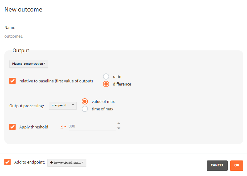
For single time-to-event outputs:
- Has event / has no event / time of event: “has event” and “has no event” calculates if the individual had or didn’t have an event during the observation period. This is a binary true/false outcome. “time of event” uses the TTE output as outcome directly. The outcome is then of type ‘time-to-event’.
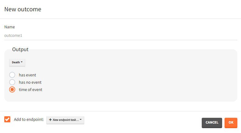
For repeated time-to-event outputs:
- Has at least one event / number of events per id / time of event #: “has at least one event” leads to a binary true/false outcome depending if the individual has at least one event during the observation period or not. “number of events per id” count the total number of events for each individual. This is an outcome of type ‘value’. “Time of event # “ generates a time-to-event outcome with a single event per individual. The index of the event to be considered can be typed-in by the user.
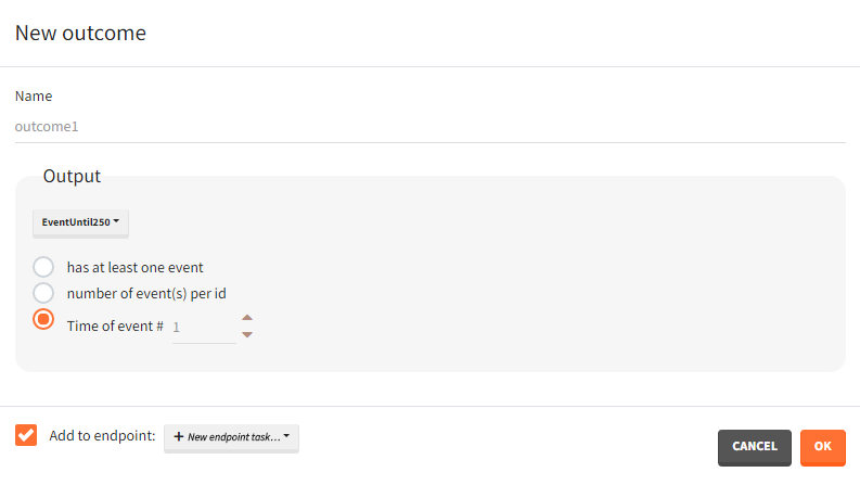
Occasions
In case occasions, you can choose to compute the outcome for each individual, or for each occasion of each individual. Select a corresponding radio button in the outcome definition window
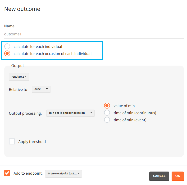
Outcomes organization
Outcomes are building blocks for endpoints. When you create a new outcome, you can add the outcome to a new or to an existing endpoint via the option “Add to endpoint” at the bottom of the outcome definition window. The Outcomes & endpoints section displays only the outcomes used in endpoints. All defined outcomes, whether used or not in an endpoint, appear in the list of outcomes:
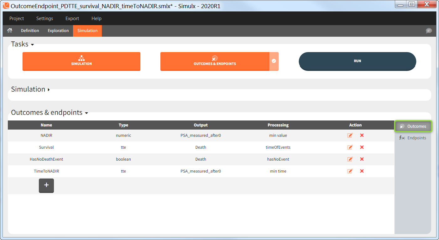
Outcomes of the same type can be combined together using AND/OR for binary true/false outcomes (e.g Cmax < threshold1 and Ctrough > threshold2), or MIN/MAX for double values and time-to-event (e.g max(CmaxParent, CmaxMetabolite) ).
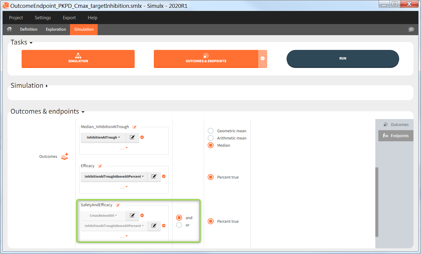
Endpoints
Endpoints summarize the outcome values over all individuals, for each simulation group and each replicate. To create a new endpoint, you can select one or several outcomes of the same type from the drop-down menu (highlighted below in blue) or click on the “+” icon next to the Endpoint header. Endpoints are also created automatically, when at the bottom of an outcome definition you select the option “Add to endpoint: New endpoint”. Once you create an endpoint, you can change its name highlighted below in green).
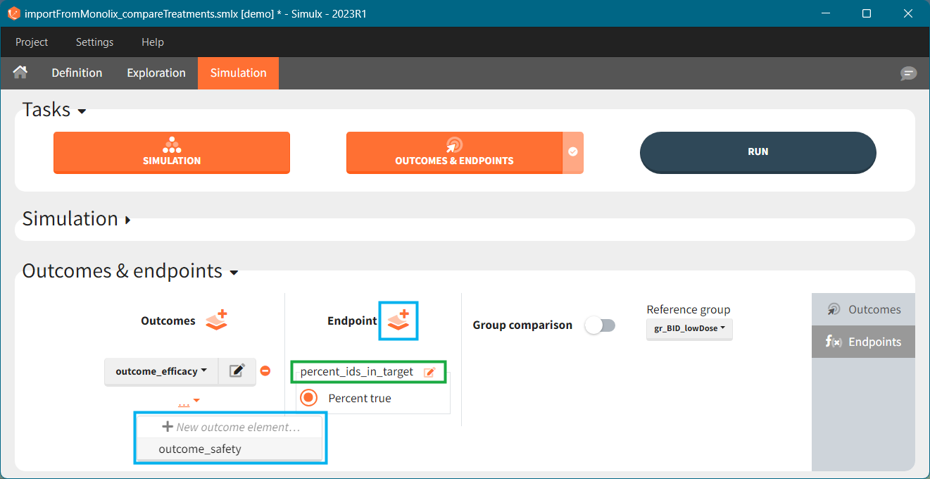
There are several options to summarize the individual outcomes into an endpoint. It depends on the type of outcomes:
- value outcomes: the endpoint can be
- geometric mean. Includes calculation of the coefficient of variation.
- arithmetic mean. Includes calculation of the standard deviation.
- median. Includes calculation of the 5th and 95th percentiles.
- binary true/false outcomes: the endpoint will be the percentage of true. Includes calculation of the “total number true”.
- time-to-event outcomes: the endpoint will be the median survival (time at which the Kaplan Meier curve is equal to 0.5). Includes calculation of the lower bound (5th) and and upper bound (95th) of the confidence interval of the median survival.
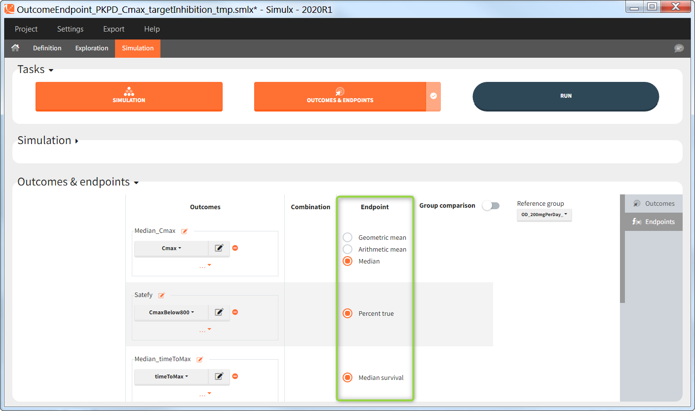
Group comparison
You can compare endpoints across simulation groups by activating the toggle “Group comparison” (green highlight). One of the simulation groups must be defined as the reference group (blue highlight) and all other groups will be compared to this reference group. For each endpoint, the group comparison can rely on a direct comparison of the endpoint values, or on a statistical test (purple highlight). The exact comparison or test applied depends on the type of the endpoint.
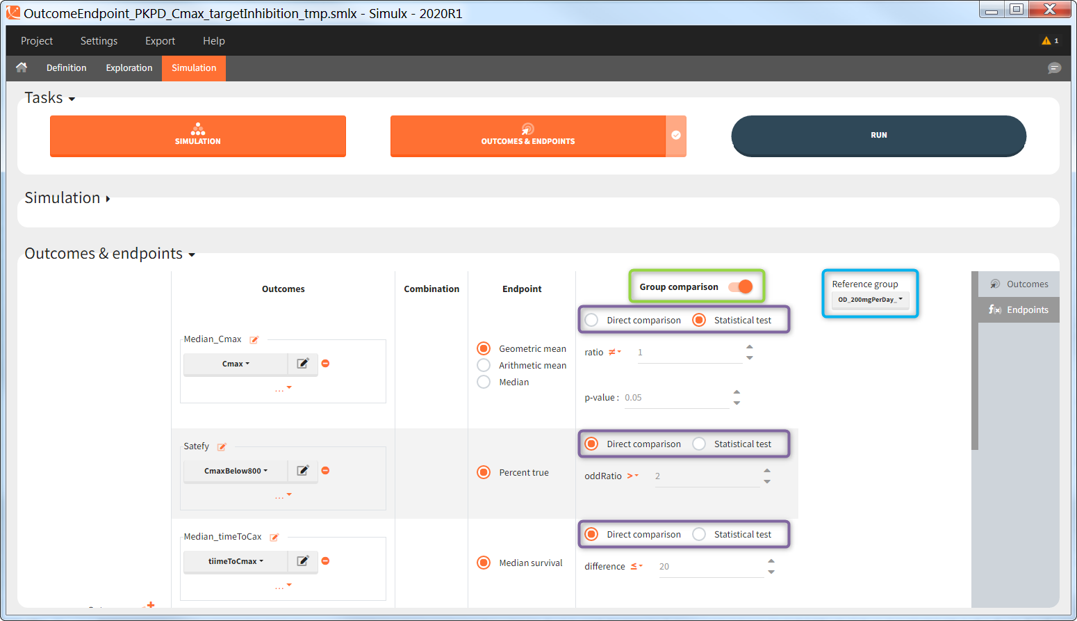
Statistical tests
This table gives an overview of the statistical tests performed in Group comparison depending on the type of outcome and endpoint. Next sections contain detailed information of each option.
| Outcome | Endpoint | Metric | Statistical test | |
| Same indiv = True | Same indiv = False | |||
| Continuous | Geometric mean | Ratio of means | Paired t-test on log-transformed |
Unpaired t-test on log-transformed |
| Arithmetic mean | Difference of means | Paired t-test | Unpaired t-test | |
| Median | Difference of medians | Wilcoxon signed rank test | Wilcoxon rank sum test | |
| Binary true/false | Percent true | Odds ratio | McNemar’s exact test | Fisher’s exact test |
| Time-to-event | Median survival | Difference in median survival | Logrank test with variance correction | Logrank test |
Endpoint “median” for value outcome
This test calculates the difference between the median of the test group and of the reference group: \( \textrm{median}_{test} – \textrm{median}_{ref} \) with \(\textrm{median}_{test}\) and \(\textrm{median}_{ref}\) the median in the test and reference group respectively.
In case of a direct comparison, this difference is compared using operators =, !=, >, >=, <, <= to a user-defined value (default: 0). When this logical comparison is true, the trial simulation is considered as ‘success’.
Example: When the direct comparison “difference > 25” is true, it means that the median in the test group is larger than in the reference group by at least 25 units (e.g ng/mL if the outcome is a peak concentration).
In case of a statistical test, a Wilcoxon rank sum test (equivalent to the Mann-Whitney test) (“Same individuals among groups” not selected) or a Wilcoxon signed rank test (“Same individuals among groups” selected) is done to compare the median of the test and reference group. “difference \(\neq\) 0” represents the alternative hypothesis H1. By default, it performs a two-sided test (sign \(\neq\)) and checks if the medians significantly differ from each other. You can define single-sided tests by choosing “>” or “<“. The minimal or maximal (depending of the direction of the test) difference can also be specified (default: 0). The statistical test results into a p-value, which is compared to a user-defined threshold (default: 0.05). If the p-value is below the threshold, the trial simulation is considered as ‘success’.
Example: When the statistical test testing the alternative H1 hypothesis “difference > 25” results into a small p-value, it means that the medians of the test and reference groups differ by more than 25 units significantly (e.g ng/mL if the outcome is a peak concentration) with a larger value for test.
Endpoint “arithmetic mean” for value outcome
This test calculates the difference between the mean of the test group and of the reference group: \( \textrm{mean}_{test} – \textrm{mean}_{ref} \) with \(\textrm{mean}_{test}\) and \(\textrm{mean}_{ref}\) the mean in the test and reference group respectively.
In case of a direct comparison, this difference is compared using operators =, !=, >, >=, <, <= to a user-defined value (default: 0). When this logical comparison is true, the trial simulation is considered as ‘success’.
Example: When the direct comparison “difference > 14 ” is true, it means that the mean in the test group is larger than in the reference group by at least 14 units (e.g ng/mL if the outcome is a peak concentration).
In case of a statistical test, it performs an unpaired t-test (“Same individuals among groups” not selected) or a paired t-test (“Same individuals among groups” selected) to compare the test and reference group. “difference \(\neq\) 0” represents the alternative hypothesis H1. By default, it performs a two-sided test (sign \(\neq\)) and checks if the two means significantly differ from each other. You can define single-sided tests by choosing “>” or “<“. The minimal or maximal (depending of the direction of the test) difference can also be specified (default: 0). The statistical test results into a p-value, and compares it to a user-defined threshold (default: 0.05). If the p-value is below the threshold, the trial simulation is considered as ‘success’.
Example: When the statistical test testing the alternative H1 hypothesis “difference > 14” results into a small p-value, it means that the means of the test and reference groups differ significantly by more than 14 units (e.g ng/mL if the outcome is a peak concentration) with a larger value for test.
Endpoint “geometric mean” for value outcome
This test calculates the ratio of the test geometric mean divided by the reference geometric mean: \( \textrm{geoMean}_{test} / \textrm{geoMean}_{ref} \) with \(\textrm{geoMean}_{test}\) and \(\textrm{geoMean}_{ref}\) the geometric mean in the test and reference group respectively.
In case of a direct comparison, this ratio is compared using operators =, !=, >, >=, <, <= to a user-defined value (default: 1). When this logical comparison is true, the trial simulation is considered as ‘success’.
Example: When the direct comparison “ratio > 2” is true, it means that the geometric mean in the test group is at least twice larger than in the reference group.
In case of a statistical test, it performs an unpaired t-test (“Same individuals among groups” not selected) or a paired t-test (“Same individuals among groups” selected) on the log-transformed values (which are assumed to follow a normal distribution) to compare the means of the test and reference group. “ratio \(\neq\) 1” represents the alternative hypothesis H1. By default, it performs a two-sided test (sign \(\neq\)) and checks if the geometric means significantly differ from each other. You can define single-sided tests by choosing “>” or “<“. The minimal or maximal (depending of the direction of the test) ratio can also be specified (default: 1). The statistical test results into a p-value, which is compared to a user-defined threshold (default: 0.05). If the p-value is below the threshold, the trial simulation is considered as ‘success’.
Example: When the statistical test testing the alternative H1 hypothesis “ratio > 2” results into a small p-value, it means that the geometric mean of the test group is significantly larger than twice the geometric mean of the reference group.
Endpoint “percent true” for binary true/false outcome
This test calculates the odds ratio between the test group and the reference group. The odds ratio definition is different depending if you use paired samples case or not.
“Same individuals among groups” not selected (unpaired samples)
The odd ratio is \( \frac{pTest}{1-pTest} / \frac{pRef}{1-pRef} \) with \(pTest\) and \(pRef\) the fraction of true outcomes in the test and reference group respectively. \(1-pTest\) represents the fraction of false outcomes.
Equivalently, you can use the following contingency table to define the odd ratio.
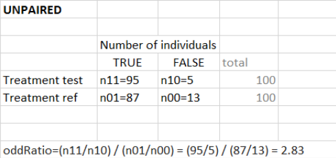
“Same individuals among groups” selected (paired samples)
In case of identical individuals among groups, the individuals which have the same outcome value in both groups (so Ref=True and Test=True, or Ref=False and Test=False) are not counted. The odd ratio is defined as\( \frac{nTest_TRef_F}{nTest_FRef_T}\), with \(nTest_TRef_F\) the number of individuals with true in the test group and and false in the reference group. It corresponds to the contingency table below. The odds ratio can frequently be zero or infinity – in particular in the absence of measurement noise – an individual true in the reference group is also necessarily true in the test group (corresponding for instance to a higher dose).
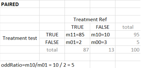
In case of a direct comparison, this odds ratio is compared using operators =, !=, >, >=, <, <= to a user-defined value (default: 1). When this logical comparison is true, the trial simulation is considered as ‘success’.
Example: When the direct comparison “odds ratio > 2” is true, it means that the odds in the test group are at least twice larger than in the reference group.
In case of a statistical test, it preforms a Fisher’s exact test (“Same individuals among groups” not selected) or a McNemar’s exact test (“Same individuals among groups” selected) to compare the results of the test and reference group via the construction of a 2×2 contingency table (which contain more information than the endpoinds \(pTest\) and \(pRef\)). “odds ratio \(\neq\) 1” represents the alternative hypothesis H1. By default, it performs a two-sided test (sign \(\neq\)) and checks if the odds ratio significantly differs from 1. You can define a single-sided tests by choosing “>” or “<“. The minimal or maximal (depending of the direction of the test) odds ratio can also be specified (default: 1). The statistical test results into a p-value, and compare it to a user-defined threshold (default: 0.05). If the p-value is below the threshold, the trial simulation is considered as ‘success’.
Example: When the statistical test testing the alternative H1 hypothesis “odds ratio > 2” results into a small p-value, it means that the odds of the test group are significantly larger than twice the odds of the reference group.
Endpoint “median survival” for time-to-event outcome
This test calculates the difference between the median survival of the test group and of the reference group: \( \textrm{medSurv}_{test} – \textrm{medSurv}_{ref} \) with \(\textrm{medSurv}_{test}\) and \(\textrm{medSurv}_{ref}\) the median survival (time at which the Kaplan-Meier estimates equals 0.5) in the test and reference group respectively.
In case of a direct comparison, this difference is compared using operators =, !=, >, >=, <, <= to a user-defined value (default: 1). When this logical comparison is true, the trial simulation is considered as ‘success’.
Example: Direct comparison “difference > 60” corresponds to median survival in the test group larger than in the reference group by 60 time units (e.g days).
In case of a statistical test, it performs a logrank test to compare the survival Kaplan-Meier curves. Selecting “Same individuals among groups”, applies a variance correction (see Jung 1999). “difference \(\neq\) 0” represents the alternative hypothesis H1. By default, it performs a two-sided test (sign \(\neq\)) and checks if the survival curves significantly differ. You can define single-sided tests by choosing “>” or “<“. For the log rank test, it is not possible to define a “minimal difference”. The statistical test gives a p-value, and compare it to a user-defined threshold (default: 0.05). If the p-value is below the threshold, the trial simulation is considered as ‘success’.
Example: When the statistical test testing the alternative H1 hypothesis “difference \(\neq\) 0” results into a small p-value, it means that the survival curves from the two groups differ significantly.
4.3.Plots
Running the tasks in Simulx automatically generates interactive plots for simulation outputs, outcomes and endpoints. Interface provides many plots features such as:
- Different chart types depending on simulation outputs and post-processing methods: individual outputs or distributions.
- Plots settings: display, binning criteria, axes, visual cues.
- Stratification and customization options.
- Export:plots as images, charts data and charts settings.
To learn more about plots in the exploration tab, click here – it is a special documentation page for the model Exploration feature.
- The Plots tab
- Continuous data
- Individual output
- Output distribution
- Non-continuous data
- Time-to-event
- Discrete data
- Individual output
- Output distribution
- Outcomes and endpoints
- Numeric outcome distribution
- Binary outcome distribution
- Endpoints distribution
- Plots features
- Settings
- Stratify
- Preferences
The Plots tab
Plots tab structure and settings in Simulx is the same as in Monolix and Pkanalix. The left panel (green frame) contains the list of available plots grouped by outcome type or by chart type. Central region displays one selected plot, for instance output distribution of Cc. Each simulation group has its own subplot. On top of the plotting area, there are layout options and a button to export current plot as an image (blue frame). The right panel is for plots settings, such as display or axis options, definition of bins or visual cues. In addition, separate sub-tabs at the bottom of this panel (red frame) allow to stratify plots data and change preferences of the plotting area.
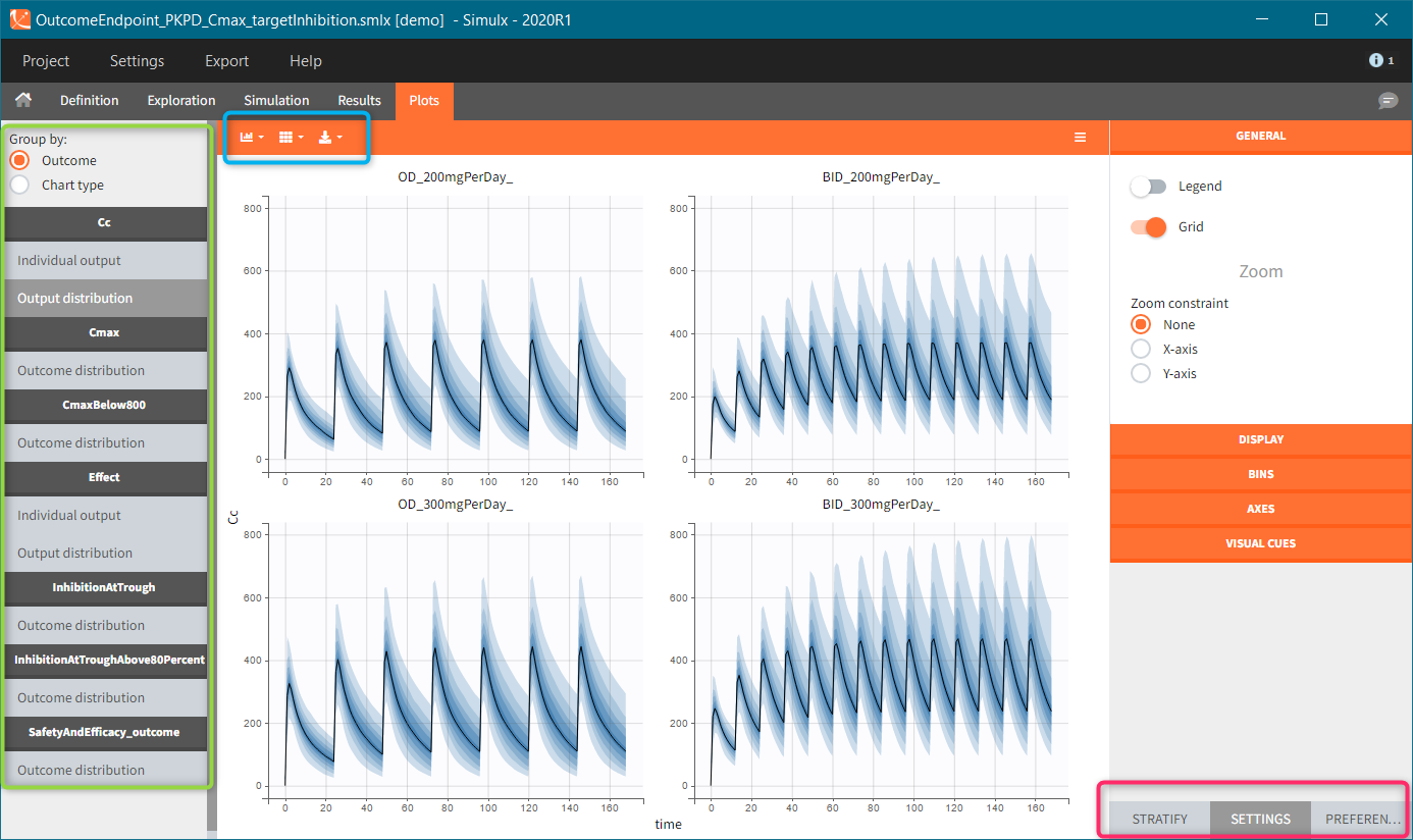
- Simulation outputs. Only output elements used in a simulation scenario generate plots. If more then one simulation output element uses the same model output, then all these simulation outputs are merged on one same plot. For instance, concentration during the whole treatment period on a fine grid and Ctrough on the last treatment day – both using model prediction Cc. Title name of the plot corresponds to the model output name.
- Outcomes. Outcomes of different endpoints have separate plots, for instance “Cmax” and “CmaxBelow800”. If there is more then one outcome in an endpoint, then a plot displays the combination of them. Moreover, it appears in the plots list as “<endpointName>_outcome”, for instance “SafetyAndEfficacy_outome”.
- Endpoints distribution is generated only for simulations with replicates.
Plots for continuous data
There are two types of plots for continuous outputs. Firstly, the individual output subplot, which contains individual curves. Secondly, the output distribution with the percentiles. Title of each outcome section in the plot list corresponds to the name of a model variable, for instance Cc for model predictions or y1 for model observations. It is not the name of the output element selected in the simulation tab.
Individual output
Individual output plots represent individual curves computed for each id and each occasion (if present in the model). It is possible to DISPLAY lines, dots and median with standard deviations (green frame), or a combination of them. The statistics (median and standard deviations) use the binning options available in the BINS section of the settings (blue frame). If simulation uses replicates, then by default a plot shows only one replicate. However, you can select other replicates – one or several – in the DISPLAY sub-tab.
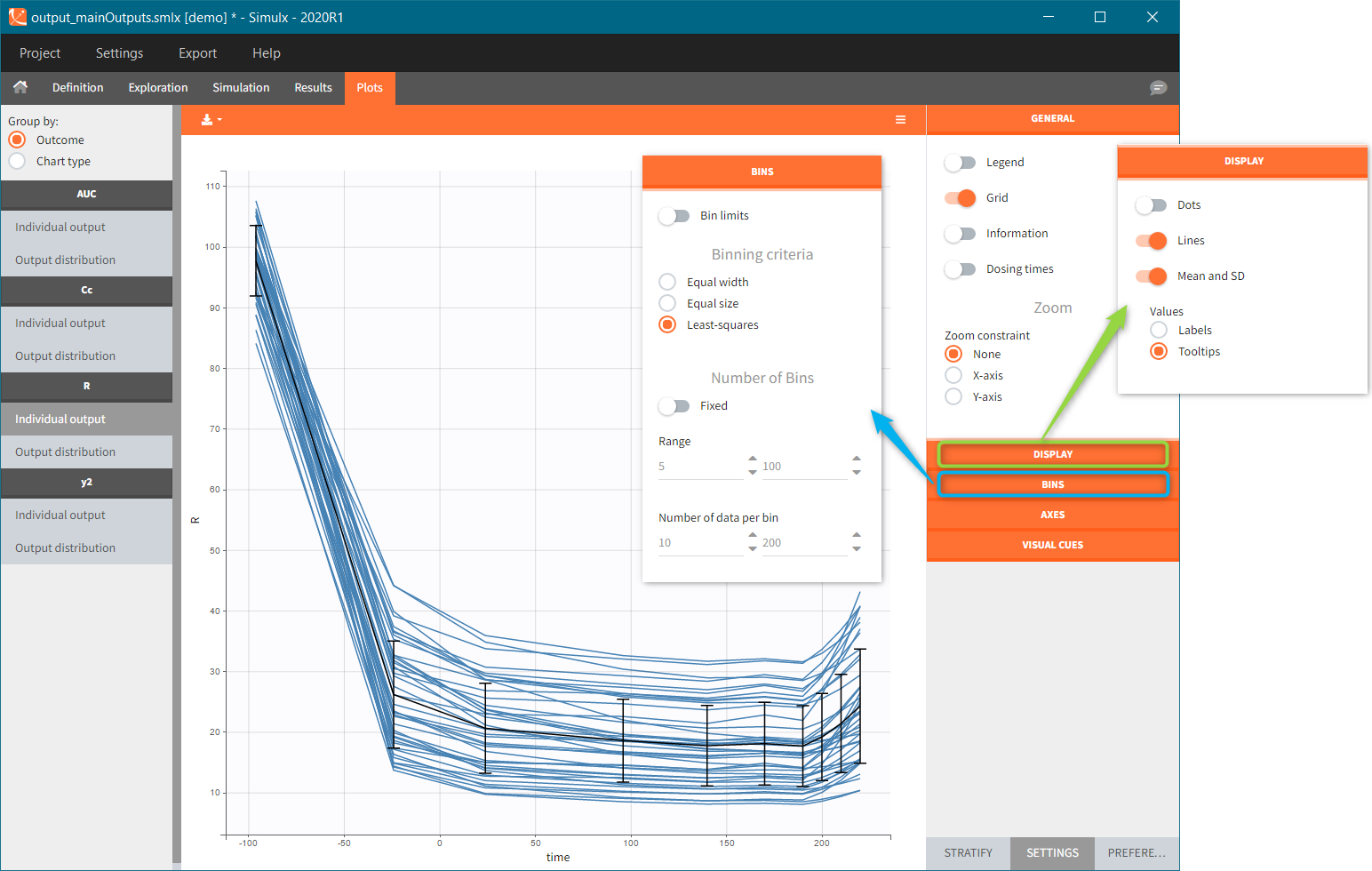
The ID used in plots stratification is the simulated ID, which is the id column in the result tables. ID i is the i-st parameter set sampled for simulation.
Since the version 2023R1, if a simulation uses elements with custom id lists, for example a table of individual treatments, or a table of individual parameters, the original ids in these tables are available to stratify the plots. For example in the demo project “importFromMonolix_useEBEs_originalID.smlx”, we use the element mlx_EBEs which is a table of individual parameters. The original IDs used in this table can be used to color or split the individual output trajectories.
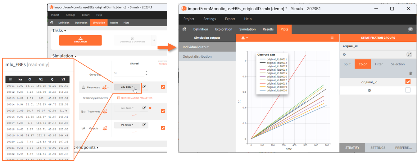
Output distribution
Output distribution plots show percentiles of the simulated data for all ids and all replicates computed. The BINS section of the settings contains the binning options. DISPLAY settings allow to change plot features, such as median, number of percentiles bands and levels.
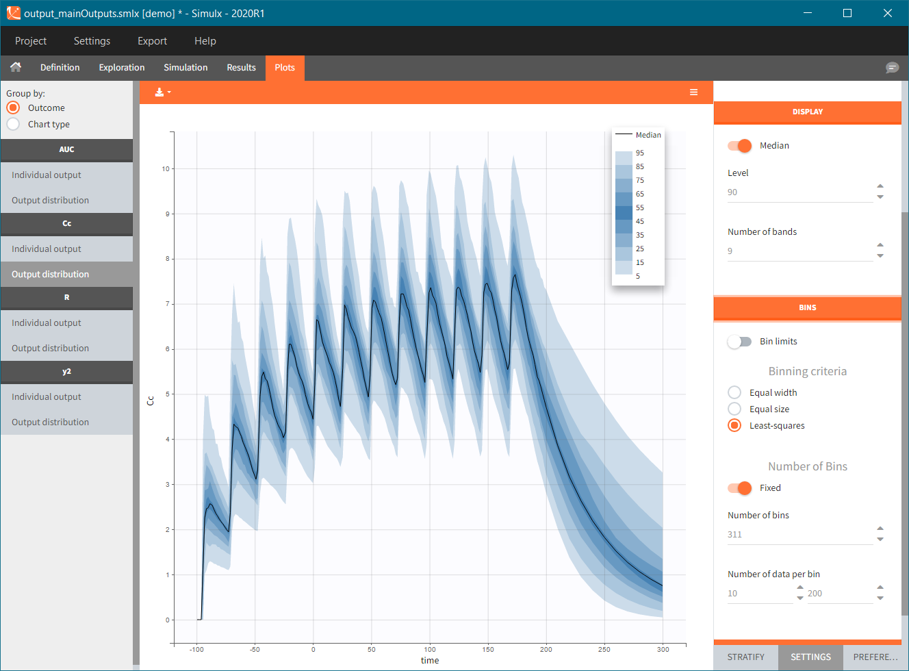
When the “Output distribution” plot is split (by simulation group or by a covariate), it is possible to overlay the prediction intervals on a single plot with different colors using the “merged splits” toggle. You can choose the colors in the “stratification groups”. This feature is available starting from the Simulx 2023 version.
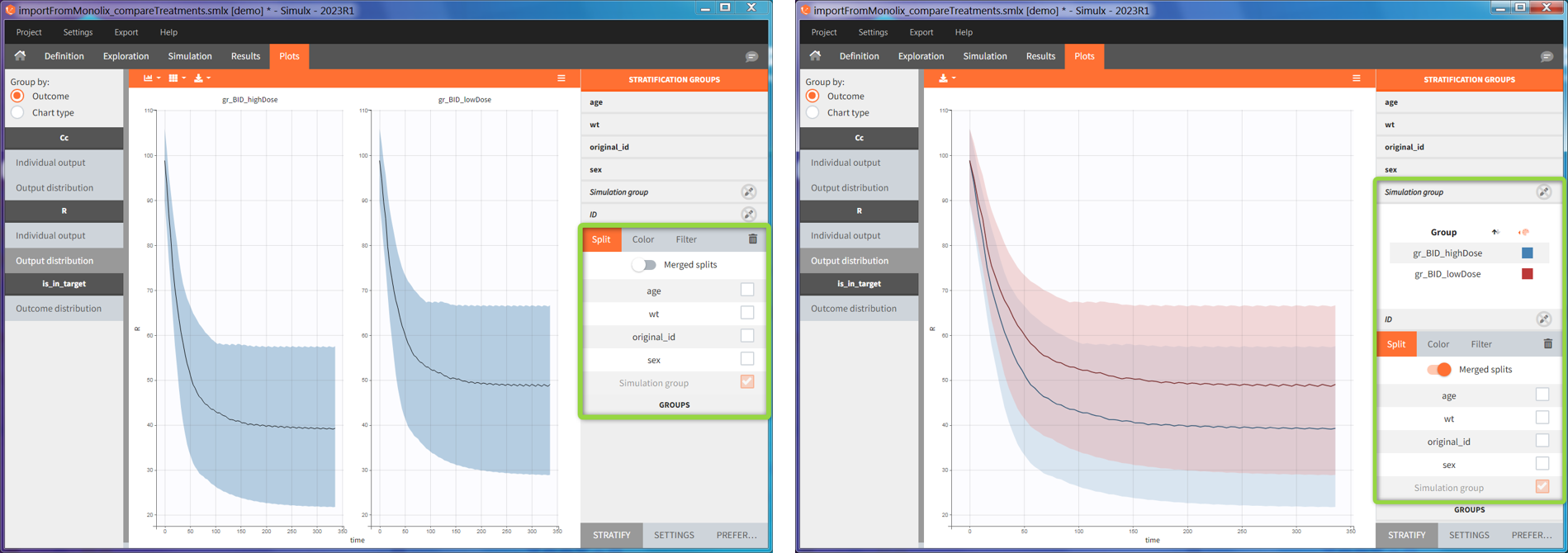
Plots for non-continuous data
Time-to-event
Individual output of time-to-event data is a single Kaplan-Meier curve – estimator of the survival function. In addition, for simulations with replicates, the Kaplan-Meier curves for each replicate are interpolated on one grid and displayed as a prediction interval at a specific level (blue frame). Mean number of subjects plot is available in the SUBPLOTS section (green frame). Click here for more information about time-to-event data plots.
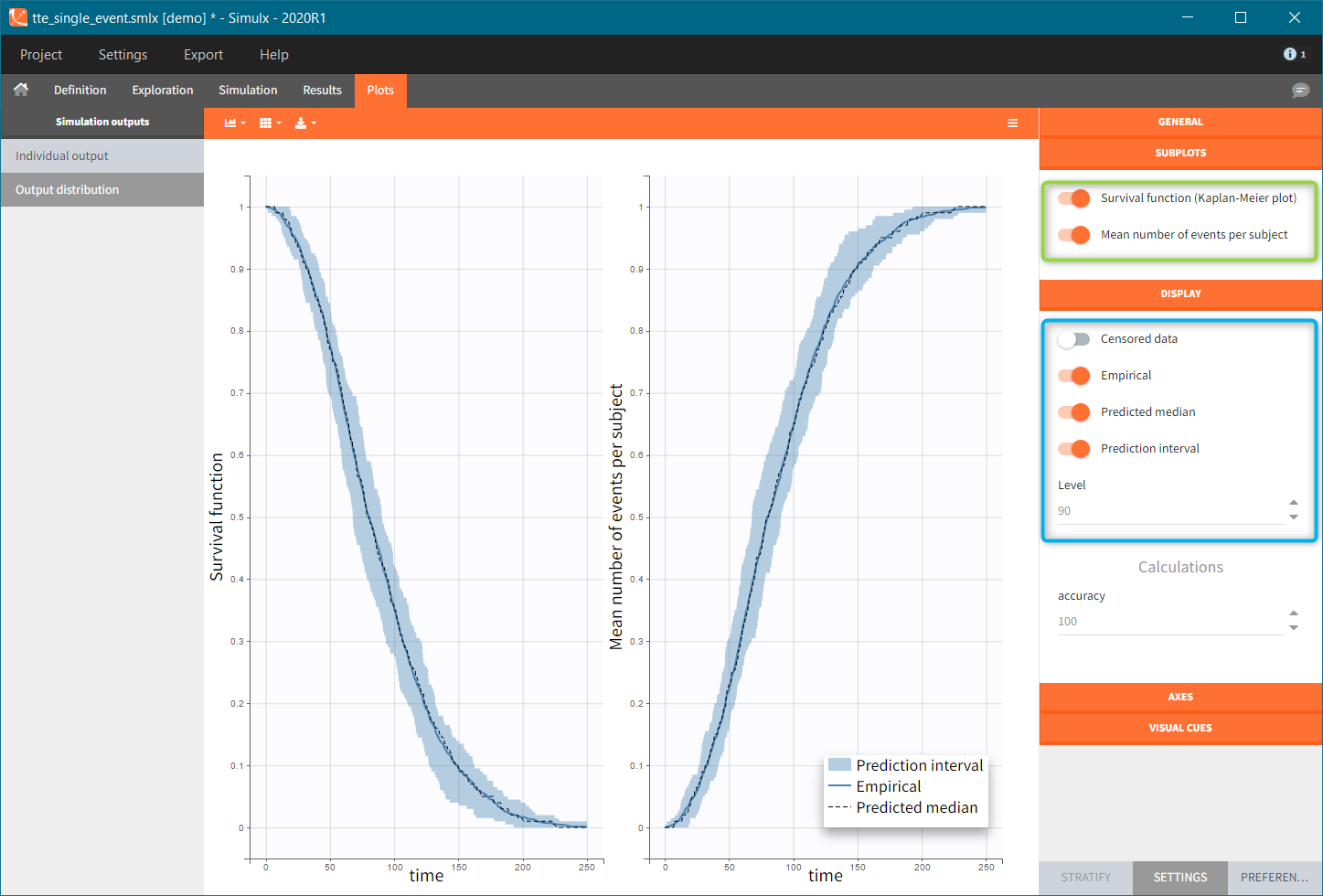
Discrete data (categorical and count)
Individual outputs are functions of time for each individual and occasion.
- Count data: plots show the number of observed events in a specific period, for instance “number of good answers” (on the left).
- Categorical data: plots show nominal categories, for instance “respiratory status level” (on the right).
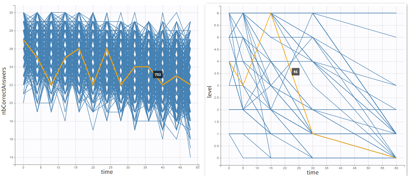
Output distribution shows the time evolution of probabilities of different categories. In case of count data, each number of “counts” constitutes a separate category.
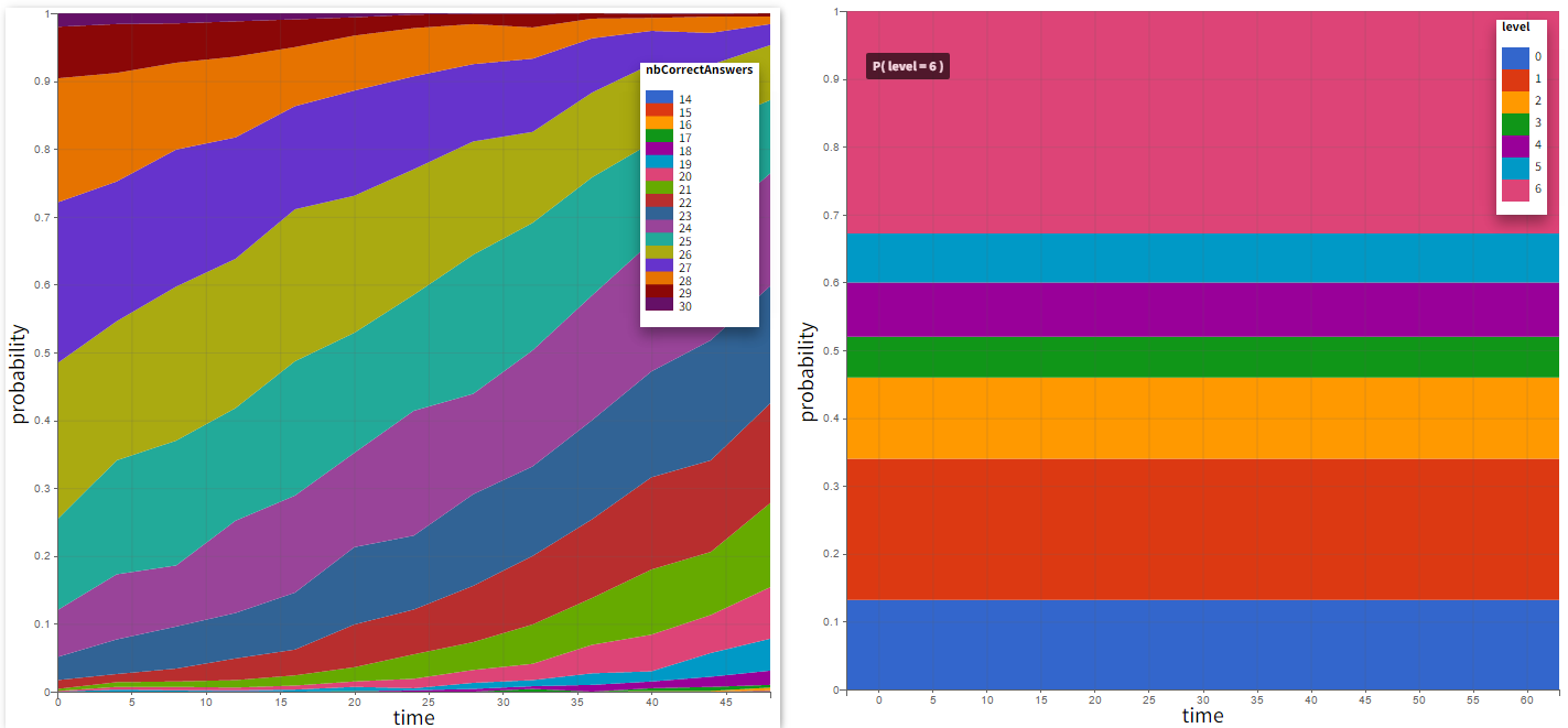
Plots for outcomes and endpoints
- Outcomes represent a post-processing of the simulation outputs done for each individual, so plots display their distribution within a population. Simulx displays only outcomes used in endpoints (Outcome&endpoint section in the simulation tab). If there are several outcomes in one endpoint, then the outcome distribution corresponds to of a combination of these outcomes, and not to separate outcomes.
- Depending on a type of an outcome, plots are histograms or box plots for numeric outcomes, and stacked histograms for binary outcomes.
- Endpoints summarize the outcome values over all individuals. In simulation with replicates, Simulx displays them as box plots.
- In all boxplots, the dashed line represents the median, the blue box represents the 25th and 75th percentiles (Q1 and Q3), and
the whiskers extend to the most extreme data points, outliers excluded. Outliers are the points larger than Q1 + w*(Q3 – Q1) or smaller than Q1 – w*(Q3 – Q1) with w=1.5. Outliers are shown with red crosses.
[Demo: 6.1.outcome_endpoint/OutcomeEndpoint_PKPD_Cmax_targetinhibition]
Numeric outcome distribution:
“Cmax” outcome gives for each individual the maximum of the output element “Plasma concentration”. In this case, the outcome distribution can be a box-plot or as a histogram (selection in the DISPLAY settings). Each group is on a separate subplot. This outcome is the only outcome in the endpoint, so the title name of the plot in the list coincides with the outcome name.
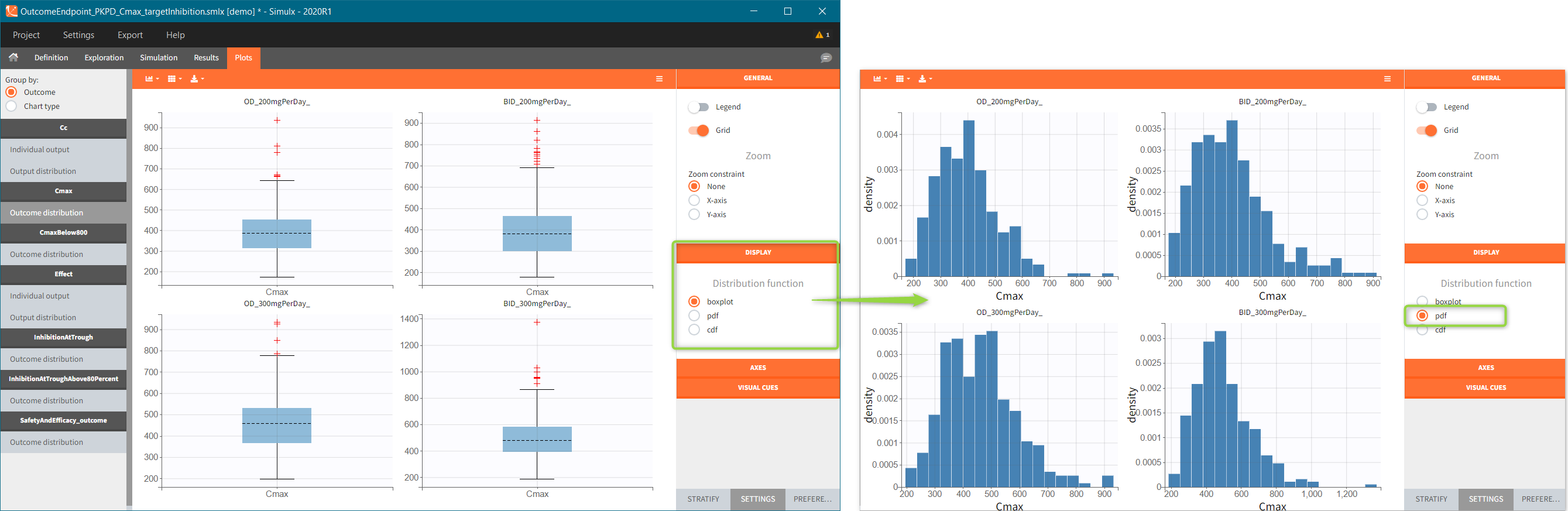
Binary outcome distribution
“CmaxBelow800” outcome is a of boolean type (true/false) and compares the maximal value of the “Plasma concentration” with a threshold of 800. If Cmax is below this value, then the outcome is true, otherwise it is false. Similarly, “inhibitionAtTroughAbove80Percent” outcome compares the average of the values in the output element “TargetInhibition_at168h” with a threshold of 0.8 (i.e 80%). These two outcomes belong to one endpoint “SafetyAndEfficacy”, so the plot shows the distribution of true/false values corresponding to the combination of the two conditions. In this case, the title name of the outcome plot is the name of the endpoint “_outcome” (red frame). Binary outcomes use stacked or grouped histograms (green frame). Hovering on a any part of the histogram highlights it, shows the outcome value and the corresponding number of individuals.
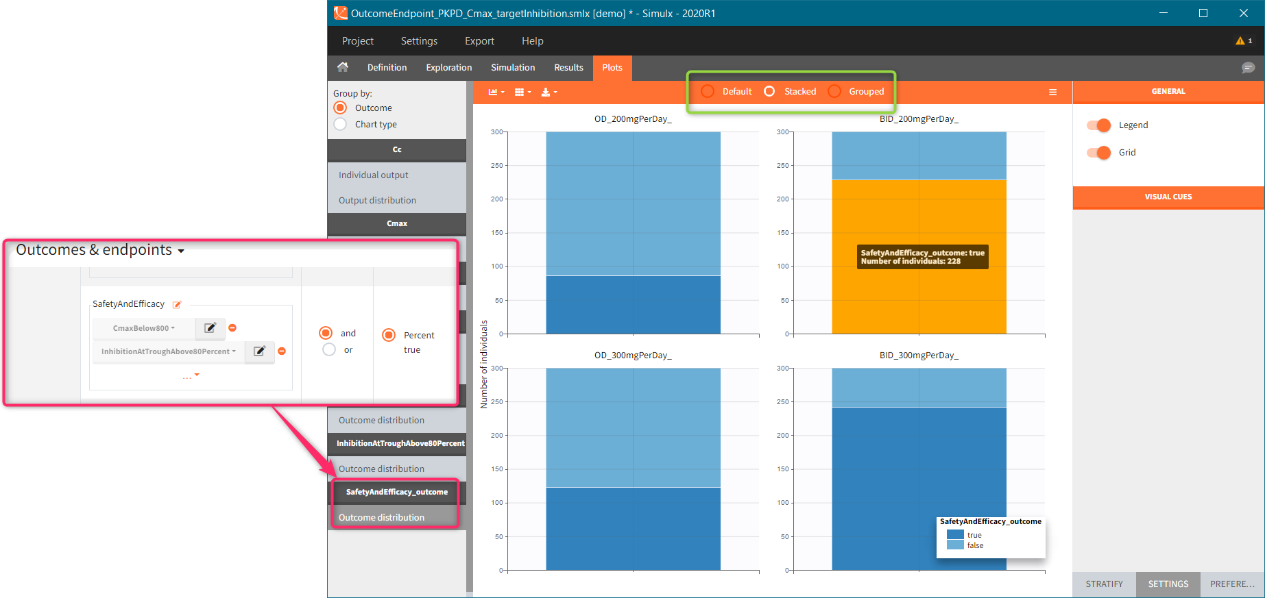
Endpoint distribution
If this simulation scenario is run several times – option “replicates” available in the Simulation section – then the endpoint distribution plots are added to the plots list. Endpoint median_Cmax is a a box-plot with median value and standard errors for groups listed on the x-axis. For endpoints using numerical outcomes, uncertainty of the 5th and 95th percentiles can be added from the settings – SUBPLOTS section (green frame).
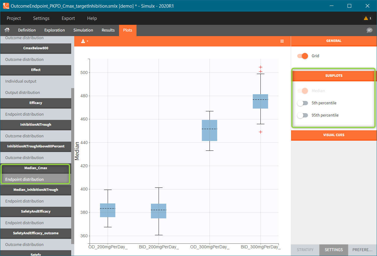
Endpoints using binary outcomes, in this example the SafetyAndEfficacy endpoint, calculate the percentage of individuals with “true” outcomes values. As previously, the endpoint distribution is a box-plots with different groups on the x-axis. A subplot with the number of individuals is available from the settings.
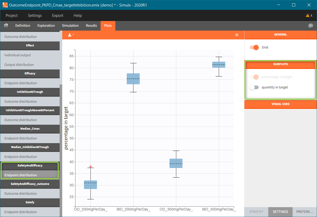
Plots features
The right panel of the Plots tab has several sub-tabs – at the bottom of the interface window – to interact and customize the charts:
- “Settings” modify plots elements, such as: hide or display additional data, adjust binning criteria, change axis or add visual cues
- “Stratify” splits, filters or colors data points using covariates.
- “Preferences” customize graphical aspects of plots such as colors, font sizes, line width or margins.
Icons at the left-top angle of the plotting area – ![]() – allow to select sub-plots for visualization, change the sub-plots layout and export the plots as a png or svg file (saved in the Chart folder in the Results). In addition, using the “Export” in the top menu saves all generated plots (Export plots), saves all data used to generate plots as txt files to re-plot them outside Simulx ( Export charts data, see here for more information) and save charts settings so that the selected customization is applied to all Simulx projects (Export charts settings as default).
– allow to select sub-plots for visualization, change the sub-plots layout and export the plots as a png or svg file (saved in the Chart folder in the Results). In addition, using the “Export” in the top menu saves all generated plots (Export plots), saves all data used to generate plots as txt files to re-plot them outside Simulx ( Export charts data, see here for more information) and save charts settings so that the selected customization is applied to all Simulx projects (Export charts settings as default).
Simulx has the same architecture of plots features, preferences and export options as Monolix. Here is an extensive documentation about it, with links to Features of the week videos that explain how to use customization in MonolixSuite applications.
Settings
Settings sub tab has several sections, which may differ between plot.
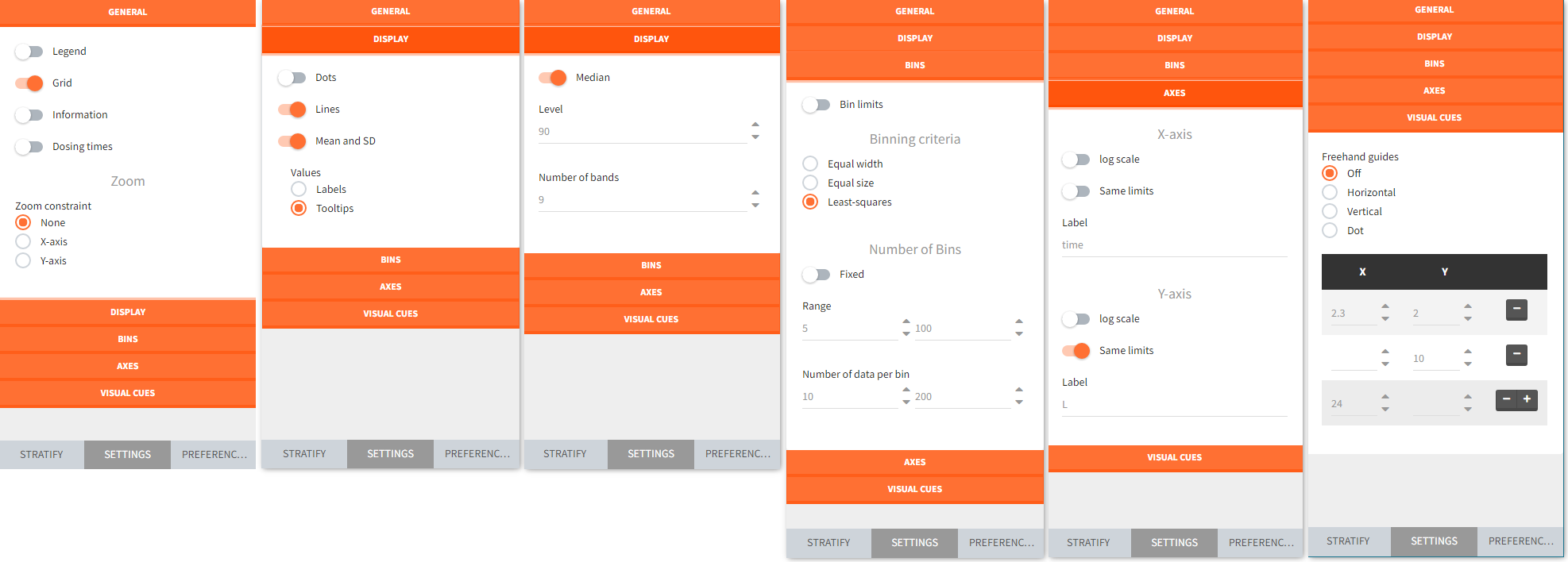
- General settings include toggle buttons add legend, data information, dosing etc. Zoom is interactive by selecting with a cursor a region directly on a plot.
- Display section for “individual output” plots has toggle buttons to add lines, data dots and Mean and SD (at least one option needs to be selected). For “output distribution” it customizes the level of percentiles and the number of bands shown.
- Bins serve to specify the criteria for computing the mean&SD for the “individual outputs” and percentiles for the “output distribution”. There are several strategies to segment the data: equal width, equal size and the least squares criterion. In addition, number of bins, range and number of data per bin are changeable.
- Axes is for general X and Y axis settings, such as log scale, same limits across plots and main axis titles.
- Visual cues freehand guides option allow to place additional lines or points on plots directly with a cursor. Definition of a specific location is via (X,Y) coordinates – one entry filled gives a line, two filled entries specify a point.
Stratify
Stratification panel contains a list of covariates that can split, color or filter the data. Simulx automatically allocates covariates in groups – according to modalities for categorical covariates and in two “equal count” groups for continuos covariates. As a result stratification is immediately applied after ticking appropriate boxes.
Example:
- Color data according to two weight groups (blue frame)
- Split data between HV (healthy volunteers) and RA (rheumatoid arthritis) patients (green frame)
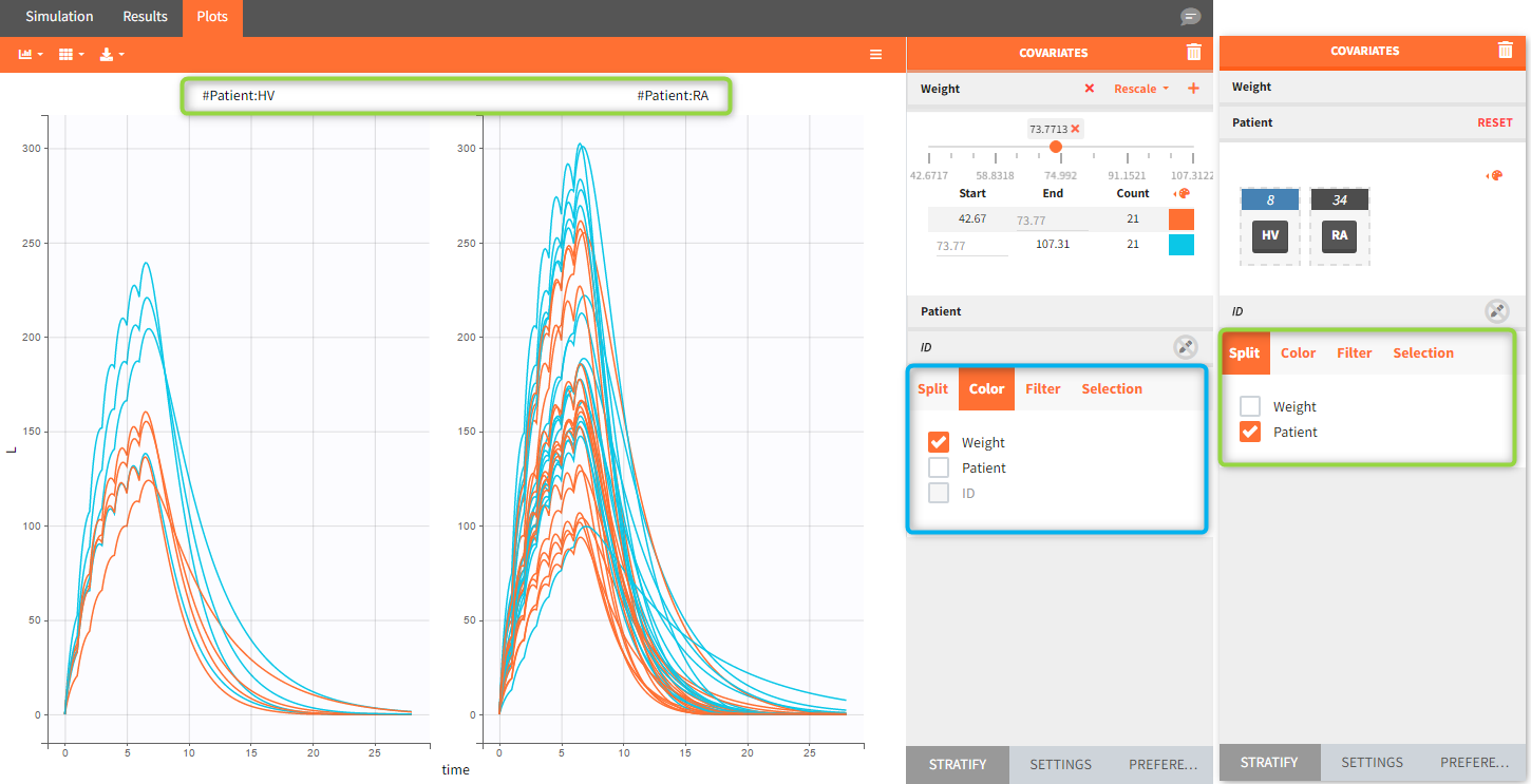
When the “Output distribution” plot is split (by simulation group or by a covariate), it is possible to overlay the prediction intervals on a single plot with different colors using the “merged splits” toggle. The colors can be chosen in the “stratification groups”. This feature is available starting from the 2023 version.
4.4.Results
The results tab displays the simulated values and the outcomes and endpoints as tables.
Result tables are organized into three sections:


Simulation
The simulation tab displays the simulated output values and the sampled individual parameters.
Outputs
Because the simulated output values are usually a very large table, the results are presented as percentiles for continuous simulations (minimum, 5th percentile, median, 95th percentile and maximum) and as percentage of survival and average number of events for time-to-event simulations. These statistics are calculated over time bins calculated automatically. When replicates are used, the statistics are calculated over all replicates merged together. Each simulation group is displayed as a separate table.
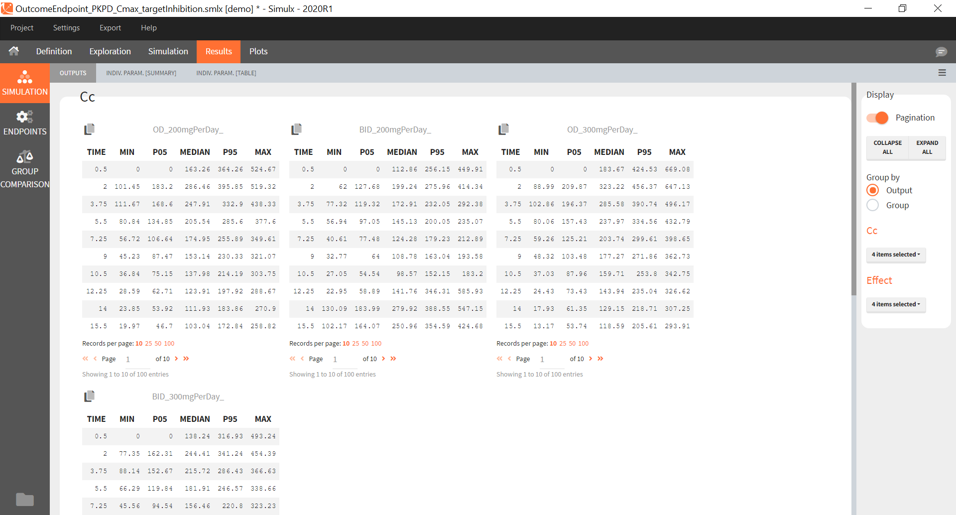
Individual parameters [Summary]
This tab displays the percentiles summarizing the distribution of individual parameters used for simulation for each of the groups. These parameters have been either directly defined by the user or sampled from the population parameters defined by the user. As for the simulated outputs, the statistics are calculated over all replicates merged together.
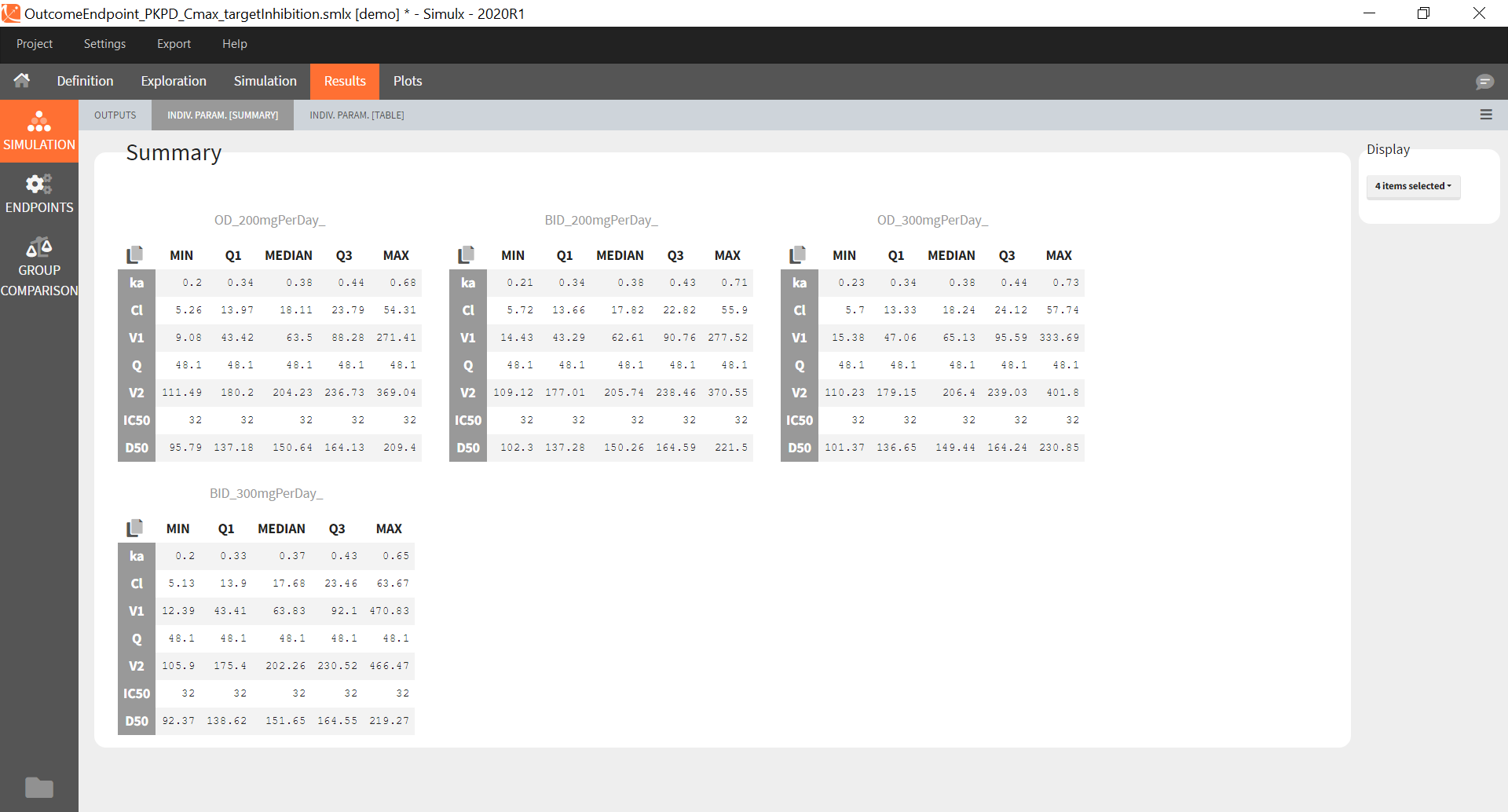
Individual parameters [Table]
This tab displays the full tables of individual parameters for all replicates and for all groups. The content of these tables can also be found in a table gathering all groups in the result folder>Simulation>individualParameters.txt .
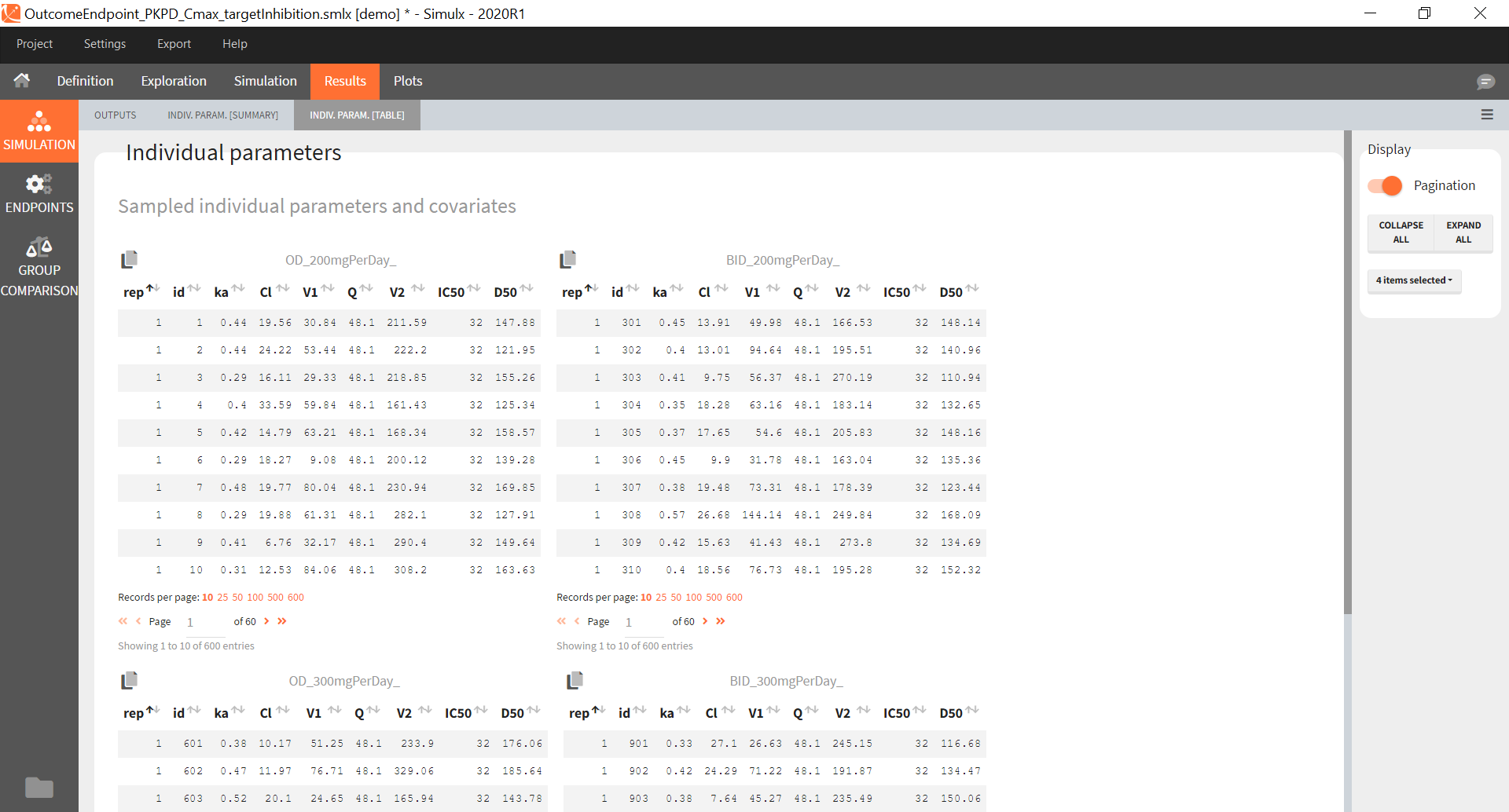
The id column in these tables is the simulated id, meaning that id i is the i-st parameter set sampled for simulation.
Since the version 2023R1, if elements using original id lists have been used for simulation, for example a table of individual treatments, or a table of individual parameters, the original ids in these tables is reported in the individual parameter tables in the “original_id” column. For example in the demo project “importFromMonolix_useEBEs_originalID.smlx”, we use the element mlx_EBEs which is a table of individual parameters. The original IDs used in this table are reported in the sampled individual parameters table, together with the simulated id. The original id is also reported in the output files.
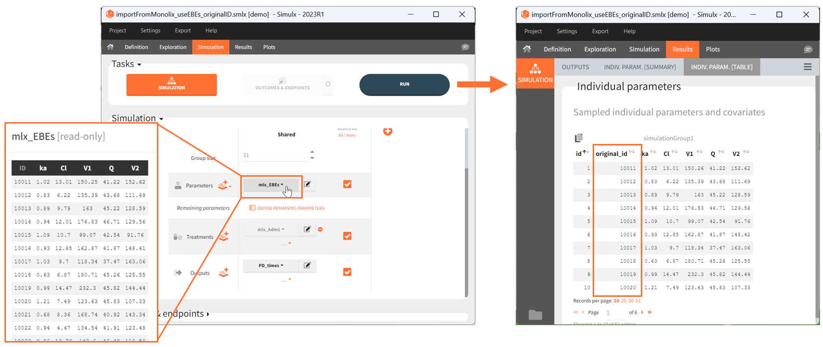
If a simulated id uses information coming from several original ids (e.g when a table a individual parameters and a table of treatment is used by the “shared ids” option is not selected), then the original id is not displayed in the GUI but it can be found in the result folder in the file ID_mapping.txt.

Endpoints
The endpoints section appears if an outcome has been defined in the simulation tab, to post-process the simulation results.
Outcomes [Summary]
The summary shows one table per outcome, displaying the percentiles over individuals and replicates for each group if the outcome is continuous, and the number of true and false individuals if the outcome is a boolean.
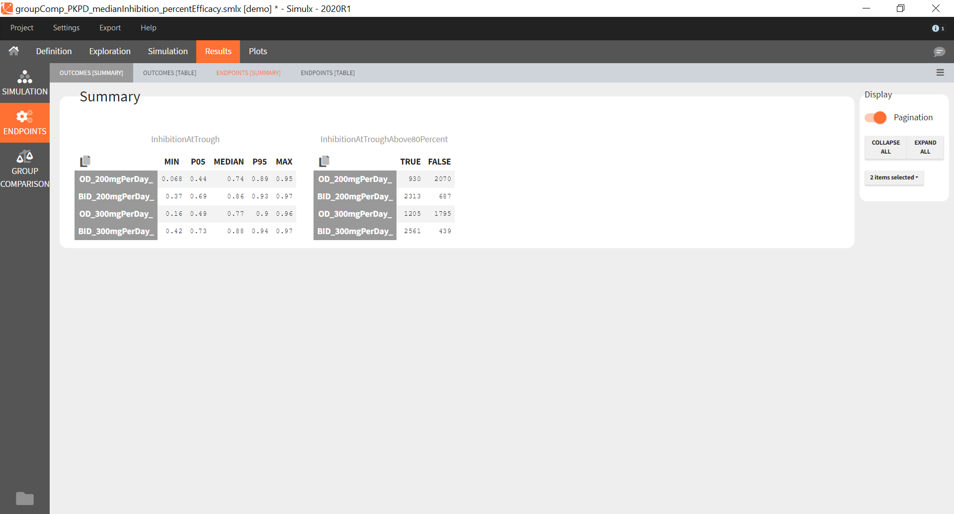
Outcomes [Table]
The outcomes table shows the outcome values for all individuals. A table of all values for each outcome also appears the result folder/Endpoints.
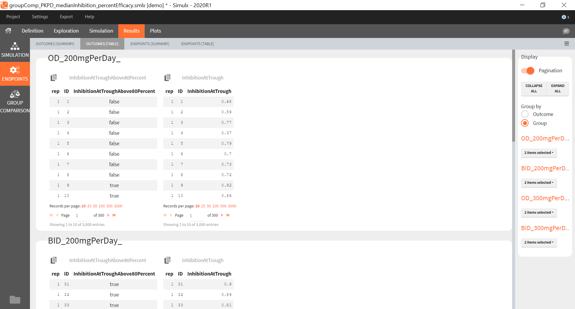
Endpoints [Summary]
Endpoints summarize the outcome values over all individuals for a specific group and replicate. The endpoints summary shows percentiles for the calculated endpoint over replicates. These percentiles give the uncertainty of the endpoint value over several clinical trial simulations.
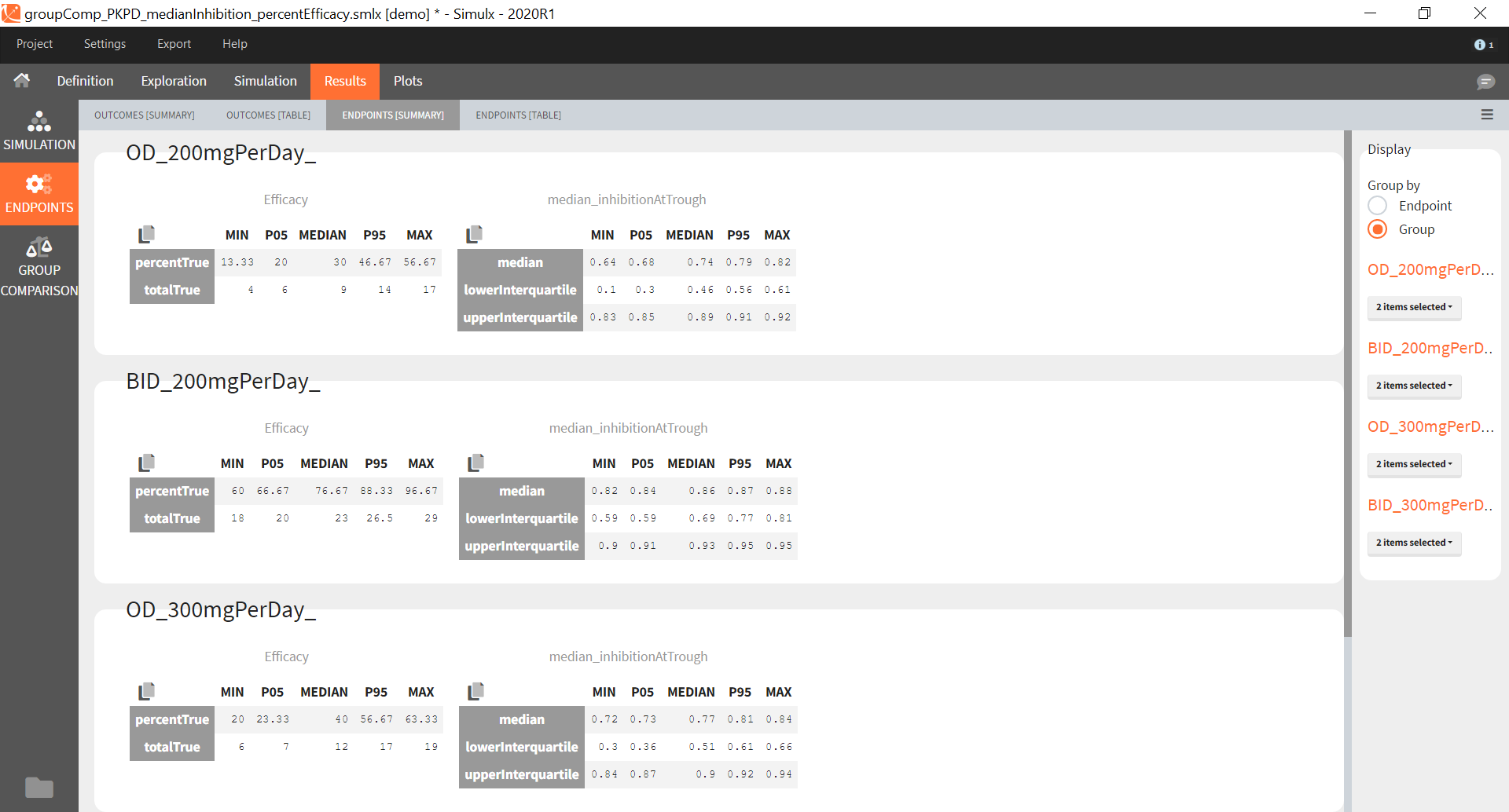
Endpoints [Table]
The endpoints table shows the value of the endpoint defined in the simulation tab for each group and each replicate. A table for each endpoint is also saved in the result folder/Endpoints.
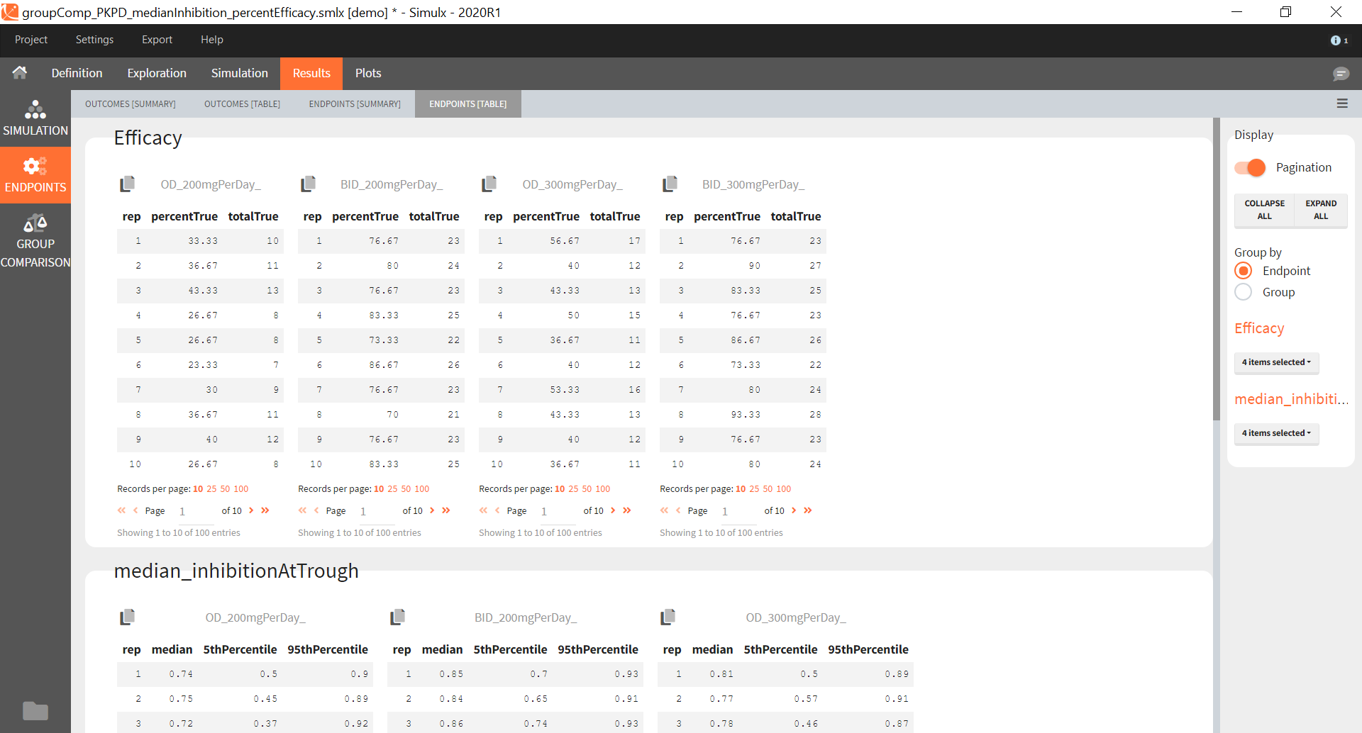
Group Comparison
If several simulation groups are used, and if group comparison is checked in the simulation tab, the group comparison section appears in the results.
Group comparison Table
For each replicate study, a test comparing the groups is performed as defined in the group comparison section of the simulation tab. The statistics of the test, p-value and the resulting decision (success or failure) according to the defined criteria are reported for each group (compared to the reference group) and for each replicate. A table is also saved for each statistical test and for each decision criterion in the result folder/Endpoints.
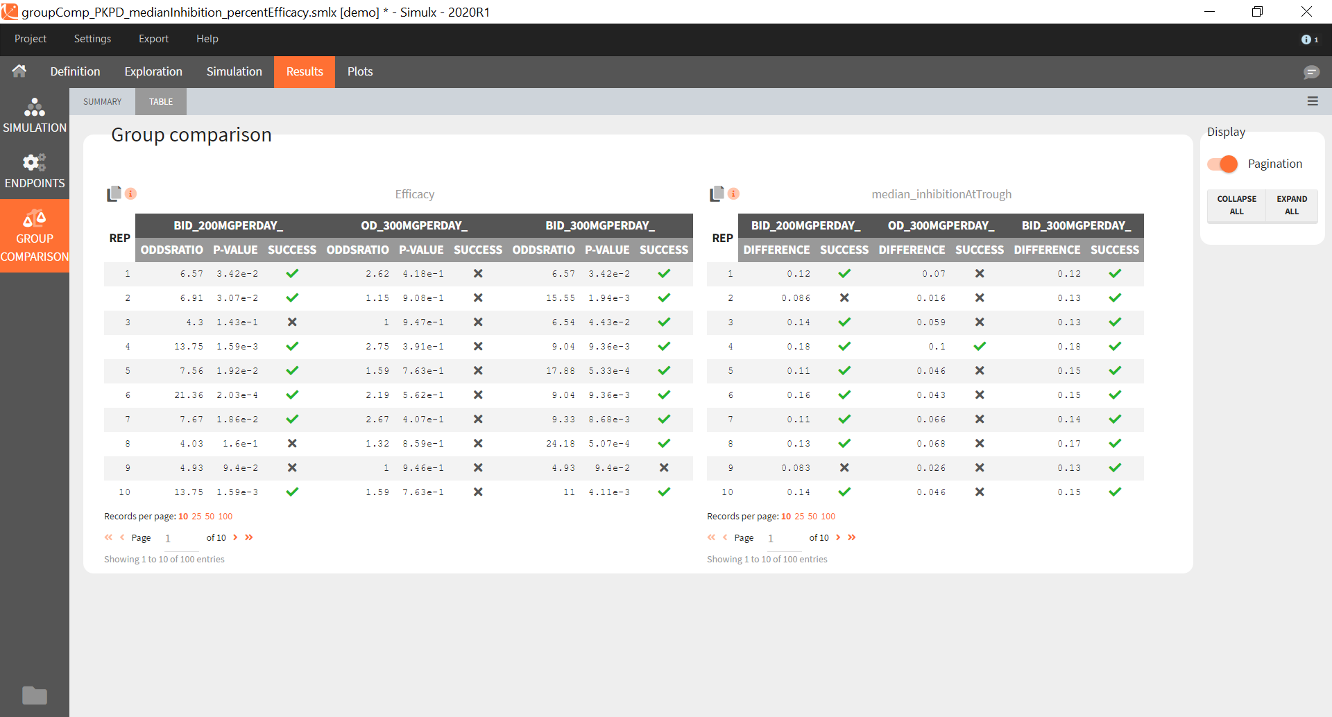
Group comparison Summary
The summary of group comparison shows for each group the percentage of replicates that led to a successful test.
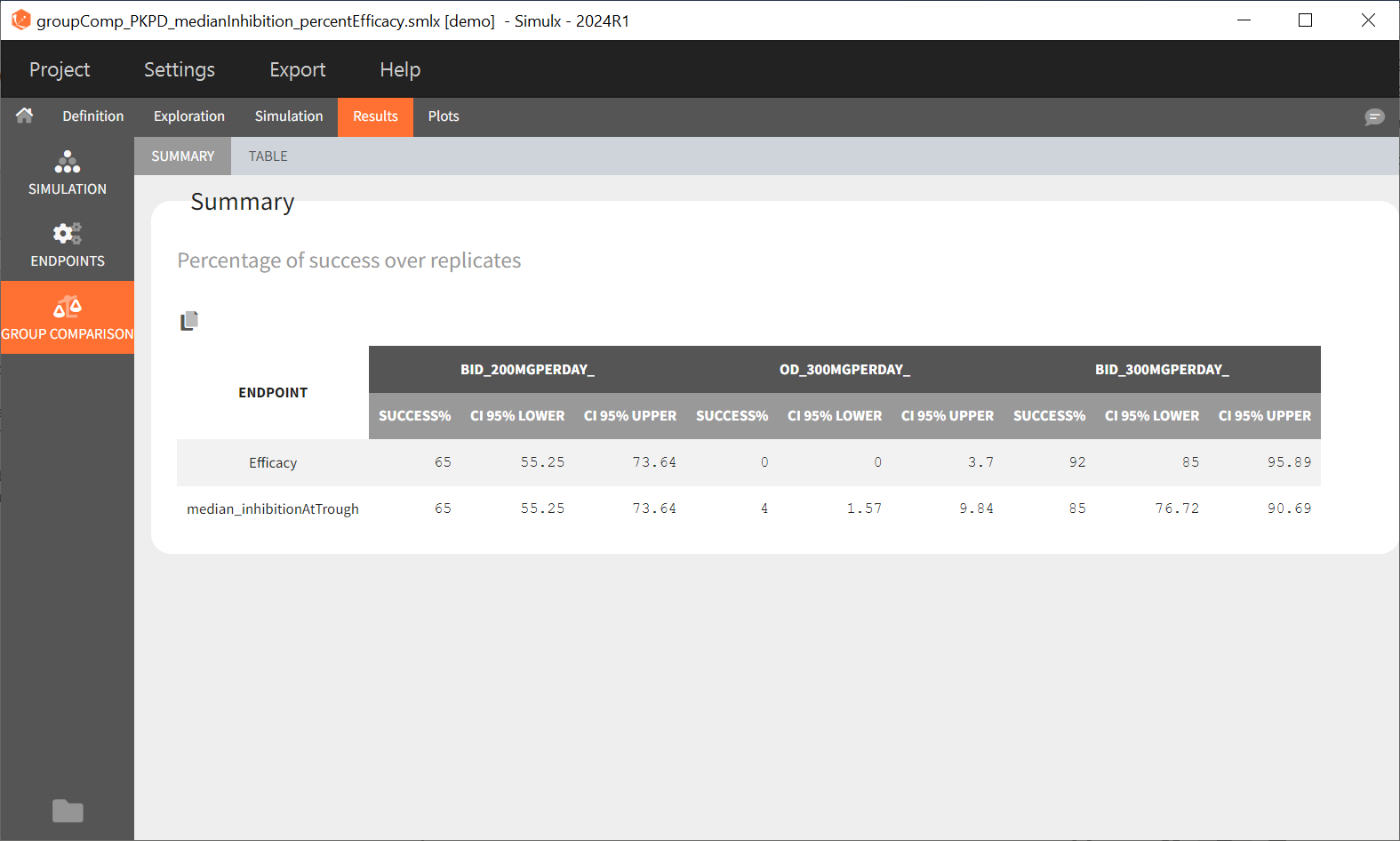
Starting from version 2024R1, the success rate across the replicates is now complemented by the corresponding confidence interval. The formula is based on the Wilson interval formula given by:
\( CI_W = \frac{X + \kappa^{2}/2}{n + \kappa ^{2}} \pm \frac{\kappa ~\sqrt{ n}}{n+ \kappa ^{2}}\sqrt{\hat{p}\hat{q}+\kappa^{2}/(4n)} \),
where \(n\) is the number of replicates, \(X\) the number of successful trials over the replicates, \( \hat{p}=\frac{X}{n}\) corresponds to the rate of successful trials, \( \hat{q} =(1-\hat{p})\) to the rate of unsuccessful trials. \( \kappa\) corresponds to the \( \alpha\) level’s \( z\) -score, where \( \alpha= \)0.05 for a 95% confidence interval.
Export Simulations
Export simulations as output files at each run
The full table of simulated values can be generated at each run if the preference setting “Export simulation files” is true. It will then appear in the result folder > Simulation > simulation_xxx.txt with xxx the output variable name.
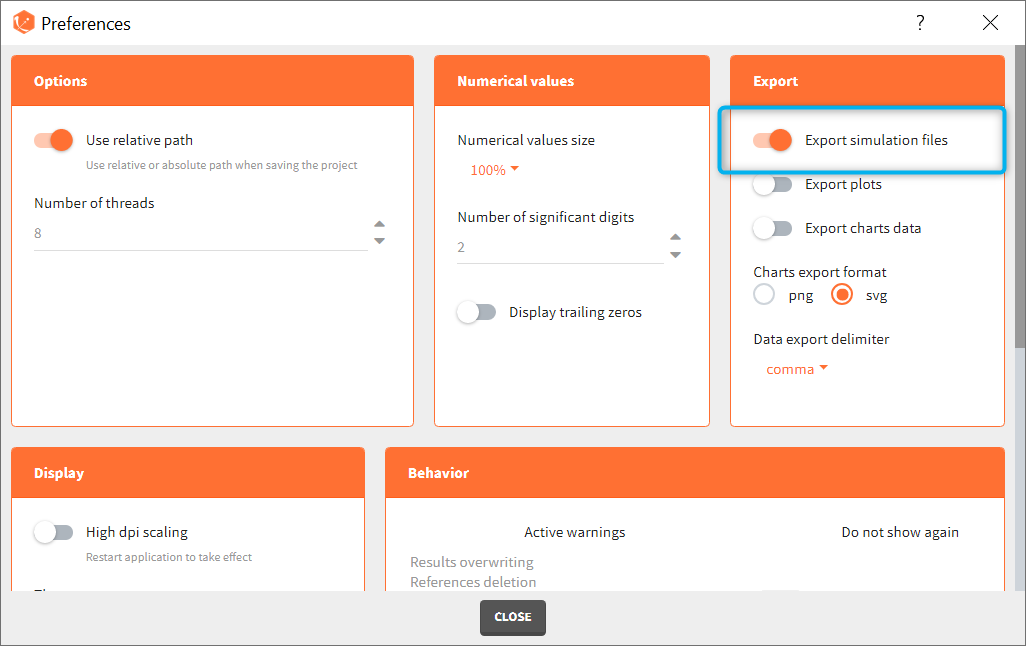
Export simulations as a Monolix or PKanalix project
Note that this option not available in Simulx versions prior to 2023.
After running simulations, it is possible to generate a new Monolix or PKanalix project using the simulated values as dataset. This can be done from the menu Export > Export project to:
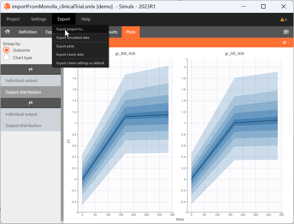
In the pop-up window, you can choose:
- to which application you want to export the simulated dataset: PKanalix or Monolix.
- names to the generated dataset (based on simulations) and generated model file (if the model is not part of the library).
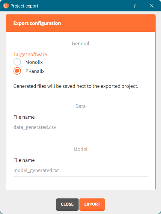
Click the “EXPORT” button at the bottom to confirm. The target application (Monolix or PKanalix) will open automatically with a predefined project called “untitled”. The simulated dataset and model files (if not from the library) will be copied next to the new new project – first in the temporary folder, when the project is “untitled”, then to the final destination, where you save the project.
The dataset in the new project will be set in the following way:
- A column ID contains the identifiers for the individuals simulated in the Simulx project. It is tagged as ID if no replicates have been used in Simulx.
- If replicates have been simulated, a UID column containing a unique identifier combining replicate and ids (eg 1_rep1) is tagged as ID, and a rep column indicates the replicate (it is possible to use filters to select a single replicate if necessary).
- If external elements have been used in Simulx, original IDs coming from these elements are indicated in a column original_id which is ignored by default, but can be tagged by the user as categorical covariate or ID, depending on the situation.
- Simulation groups are given in a column group tagged as stratification categorical covariate.
- If several model outputs are simulated, the output names are indicated in an obsid column tagged as observation ID.
- Pre-defined tagging is used for time, observation, amount, and simulated covariates.
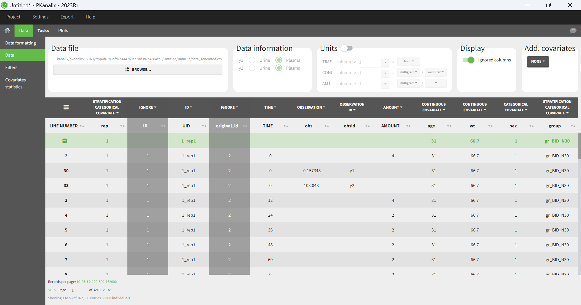
For an export to PKanalix, the new project will be set in the following way:
- the data is set as described above.
- NCA settings: default PKanalix settings for administration type, integral method, treatment of BLQ values, parameters
- NCA settings: “observation ID to use” set to the first one alphabetically (if obsid are strings) or numerically (if obsid are integers).
- Acceptance criteria: not selected.
- Bioequivalence: default PKanalix settings
- the structural model is set to the generated model file attached to the new project, or a model from the library if the Simulx project used a library model.
- The generated structural model only includes the [LONGITUDINAL] block of the Simulx model, without the error model.
- If a statistical model was used in simulx (observation or individual model), it is not included in the generated model file for PKanalix.
- The mapping automatically links the simulated observations to the model outputs.
- If additional lines were used in the Simulx project, they are added at the end of the generated structural model file.
- If output elements are defined based on intermediate variables of the model in the Simulx project, they are added to the output section of the model.
- The mapping automatically links the simulated observations to the model outputs. If a statistical model was used in simulx (observation or individual model), it is not included in the generated model file for PKanalix. The generated model only includes the [LONGITUDINAL] block without DEFINITION section.
- CA initial parameter values: set to default
- CA parameters constraints: none for normally distributed parameters, positive for log-normally distributed parameters; bounded with limits imported from the Monolix project for logit-normally and probit-normally distributed parameters.
- CA calculations settings: default PKanalix settings
For an export to Monolix, the project will be set in the following way:
- the data is set as described above.
- the structural model is set to the generated model file attached to the new project, or a model from the library if the Simulx project used a library model.
- The generated structural model only includes the [LONGITUDINAL] block of the Simulx model, without the error model.
- The mapping automatically links the simulated observations to the model outputs.
- If additional lines were used in the Simulx project, they are added at the end of the generated structural model file.
- If output elements are defined based on intermediate variables of the model in the Simulx project, they are added to the output section of the model.
- Initial values are set to default.
- the observation model and individual model in Monolix statistical model tab is set based on the Simulx project, if a statistical model was defined in the model of the Simulx project (INDIVIDUAL, COVARIATE blocks or error model in the LONGITUDINAL block). Note that the statistical model is not included in the generated model file for Monolix, but it is taken into account in the statistical model tab. Only the Monolix style syntax for the INDIVIDUAL block can be imported to the Monolix project, not the flexible style. When modifications are done to the model for compatibility reasons, Simulx warns you at export to double check the model interpretation in the Monolix project.
- if some part of the statistical model is not defined in the Simulx project, it is set to default in the statistical model tab.
Export simulations as a formatted dataset
Note that this option not available in Simulx versions prior to 2021.
To export simulations as a formatted dataset for further investigations outside the Monolixsuite, it is possible to use the menu Export > Export simulated data. This data set contains the dose, occasions, covariate, simulation groups, observation id informations in addition to the id, time and simulated values. The exported simulated data file is located in the result folder > Simulation > simulatedData.txt.
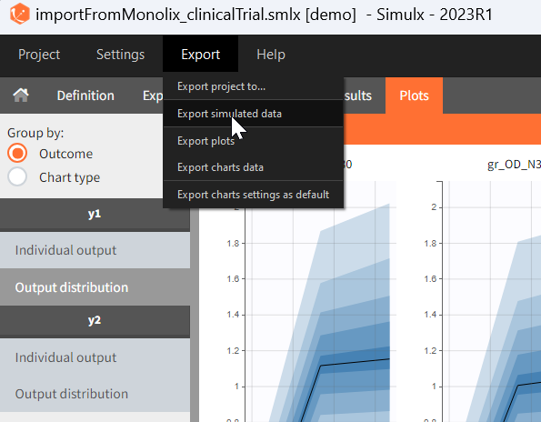
Share a Simulx project
The 2024 version of MonolixSuite introduces a highly convenient method for sharing projects. Simply click on “Share Project” in the export menu, and a zip folder is generated containing all the required files to re-open the project (dataset if applicable, model if applicable, external files if applicable, smlx file, result folder). By default, the suggested location for the zipped shared project matches that of the original, but this can be easily modified to any other location on the computer.
General display options
The tables generally contain many rows and are by default paginated. The page displayed and the number of records per page can be changed at the bottom (green highlight). The ![]() panel on the right (blue highlight) allows to switch the pagination off in order to show the entire table. The tables can also be all expanded and collapsed. When several groups and several output variables/outcomes/endpoints have been defined, the tables can be grouped by either simulation group or output/outcome/endpoint to easily compare the tables of interest. Finally it is possible to hide some of the simulation groups using the drop-down selection menu. The display panel can be hidden with the button
panel on the right (blue highlight) allows to switch the pagination off in order to show the entire table. The tables can also be all expanded and collapsed. When several groups and several output variables/outcomes/endpoints have been defined, the tables can be grouped by either simulation group or output/outcome/endpoint to easily compare the tables of interest. Finally it is possible to hide some of the simulation groups using the drop-down selection menu. The display panel can be hidden with the button ![]() at the top right. The button
at the top right. The button ![]() on the bottom left opens the result folder which contains the simulated values and their post-processing as text files. All tables can be copied to the clipboard using the button
on the bottom left opens the result folder which contains the simulated values and their post-processing as text files. All tables can be copied to the clipboard using the button ![]() at the top left . Only the displayed page is copied. To copy the entire table, expand it first.
at the top left . Only the displayed page is copied. To copy the entire table, expand it first.
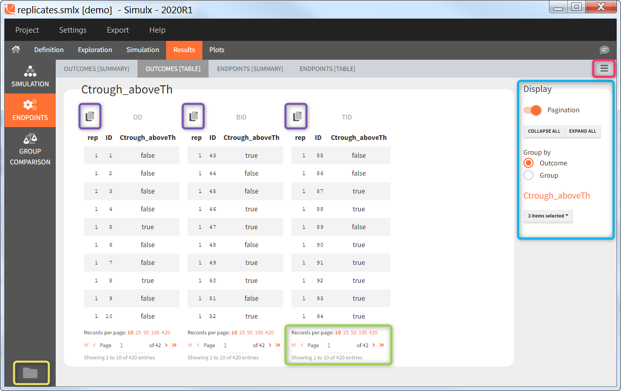
5.Simulx API
On the use of the R-functions
We now propose to use Simulx via R-functions. The package lixoftConnectors provides access to the project exactly in the same way as you would do with the interface. All the installation guidelines and initialization procedure can be found here. All the functions are described below.
- Installation guidelines and initialization procedure
- Page with typical examples
- Load a project and run the simulation
- Import a Monolix project and simulate a new output variable with the EBEs
- Create a Simulx project from scratch and simulate covariate-dependent treatments
- Import a Monolix project and simulate with new output times
- Run a simulation with different sample sizes and plot the power of the study based on an endpoint
- Handling of warning/error/info messages
Minimal examples based on demo projects are also included in the documentation of the functions below.
- List of the R functions
- Description of the functions concerning the element definition
- Description of the functions concerning the group comparison
- Description of the functions concerning the initialization and path to demo projects
- Description of the functions concerning the model extension
- Description of the functions concerning the project management
- Description of the functions concerning the project settings and preferences
- Description of the functions concerning the results
- Description of the functions concerning the scenario
List of the R functions
Description of the functions concerning the element definition
- defineCovariateElement: Define or edit a covariate element.
- defineEndpoint: Define or edit an endpoint.
- defineIndividualElement: Define or edit an element of individual parameters.
- defineOccasionElement: Define the occasion structure of the project.
- defineOutcome: Define or edit an outcome.
- defineOutputElement: Define or edit an output element.
- definePopulationElement: Define or edit an element of population parameters.
- defineRegressorElement: Define or edit a regressor element.
- defineTreatmentElement: Define or edit a treatment element.
- deleteElement: Delete an element of any type.
- deleteEndpoint: Delete an endpoint.
- deleteOccasionElement: Delete the occasion element.
- deleteOutcome: Delete an outcome.
- getCovariateElements: Get the list of all available covariate elements in the loaded project.
- getEndpoints: Get the list of all endpoints.
- getIndividualElements: Get the list of all available individual parameters elements for the simulation.
- getOccasionElements: Get the content of the occasion element that will be used for the simulation.
- getOutcomes: Get the list of all available outcomes.
- getOutputElements: Get the list of all available output elements for simulation.
- getPopulationElements: Get the list of all available population parameters elements for the simulation.
- getRegressorElements: Get the list of all available regressor elements for simulation.
- getRegressorsSettings: Get the regressors global settings.
- getTreatmentElements: Get the list of all available treatments elements for the simulation.
- setRegressorsSettings: Edit the regressors global settings.
Description of the functions concerning the group comparison
- getGroupComparisonSettings: Set settings related to the comparison of endpoints across groups.
- setGroupComparisonSettings: Set settings related to the comparison of endpoints across groups.
Description of the functions concerning the initialization and path to demo projects
- initializeLixoftConnectors: Initialize lixoftConnectors API for a given software.
- addIndividualBlock: Add an INDIVIDUAL block to a structural model.
- getDemoPath: Get the path to the demo projects.
Description of the functions concerning the model extension
- getAddLines: Get the lines that were added to a model with
setAddLines(or in the GUI). - setAddLines: Add equations to the structural model.
Description of the functions concerning the project management
- exportProject: Export the current project to another application of the MonolixSuite, and load the exported project.
- getLibraryModelContent: Get the content of a library model.
- getLibraryModelName: Get the name of a library model given a list of library filters.
- getStructuralModel: Get the model file for the structural model used in the current project.
- importProject: Import a Monolix or a PKanalix project into the currently running application initialized in the connectors.
- isProjectLoaded: Get a logical saying if a project is currently loaded.
- loadProject: Load a project in the currently running application initialized in the connectors.
- newProject: Create a new project.
- saveProject: Save the current project as a file that can be reloaded in the connectors or in the GUI.
- shareProject: Create a zip archive file from current project and its results.
Description of the functions concerning the project settings and preferences
- getConsoleMode: Get console mode, ie volume of output after running estimation tasks.
- getPreferences: Get a summary of the project preferences.
- getProjectSettings: Get a summary of the project settings.
- setConsoleMode: Set console mode, ie volume of output after running estimation tasks.
- setPreferences: Set the value of one or several of the project preferences.
- setProjectSettings: Set the value of one or several of the settings of the project.
Description of the functions concerning the results
- exportSimulatedData: Export the simulated dataset into a MonolixSuite compatible format.
- getEndpointsResults: Get the results of the outcomes & endpoints task.
- getSimulationResults: Get the results of the simulation.
Description of the functions concerning the scenario
- computeChartsData: Compute (if needed) and export the charts data of a given plot or, if not specified, all the available project plots.
- getScenario: Get the list of tasks that will be run at the next call to
runScenario. - runScenario: Run the scenario that has been set with
setScenario. - setScenario: Clear the current scenario and build a new one from a given list of tasks.
- addGroup: Add a new simulation group.
- getGroupRemaining: Get the values of the remaining parameters (typically the error model parameters) for a group.
- getGroups: Get the list of simulation groups and elements in each group.
- getNbReplicates: Get the number of replicates of the simulation.
- getSameIndividualsAmongGroups: Get the information if the same individuals are simulated among all groups.
- getSamplingMethod: Get which sampling method is used for the simulation.
- getSharedIds: Get the element types that will share the same individuals in the simulation.
- removeGroup: Remove a simulation group.
- removeGroupElement: Remove an element from a simulation group.
- renameGroup: Rename a simulation group.
- runEndpoints: Run the endpoints task.
- runSimulation: Run the simulation task.
- setGroupElement: Set the new element of a specific group.
- setGroupRemaining: Set the values of the remaining parameters (typically the error model parameters) for a group.
- setGroupSize: Define the size of a simulation group.
- setNbReplicates: Define the number of replicates of the simulation.
- setSameIndividualsAmongGroups: Define if the same individuals will be simulated among all groups.
- setSamplingMethod: Define which sampling method is used for the simulation.
- setSharedIds: Select the element types that will share the same individuals in the simulation.
- printOutcomesEndpoints: Get all the outcomes and endpoints defined in the Simulx project.
- printSimulationSetup: Get all the elements used in simulation setup: content of simulation groups and simulation settings.
[Simulx] Define covariate element
Description
Define or edit a covariate element.
Covariate elements are defined and used for simulation as in Simulx GUI. As for other elements, the covariate elements can be defined or imported, and they are saved with the Simulx project if calling saveProject. Once a covariate element is defined, it needs to be added to a simulation group with setGroupElement to be used in simulation.
Usage
defineCovariateElement(name, element)
Arguments
name |
(character) Element name. |
element |
(character or dataFrame or list) Element definition from external file path or data frame with covariates as columns, or list to select the sheet of an excel file:
|
Details
Covariate elements can be defined only if the model used in the Simulx project contains a block [COVARIATE].
A covariate element can be defined as an external file (csv, xlsx, xlsx, sas7bdat, xpt or txt) or as a data frame.
In any case, it can contain columns occasions (optional), and it should contain one column per covariate (mandatory). Covariate names and categorical covariate values must correspond to covariates and categories defined in the model (block [COVARIATE]). The occasion headers must correspond to the occasion names defined in the occasion element.
A data frame can be used only to define covariate elements of type ‘common’, i.e the same for all individuals (potentially occasion-wise). If you want to define subject-specific covariates, use an external file with an "id" column. Covariate definition with distributions is only possible in the GUI (in R, please sample from the desired distribution to generate an external file).
An external file can be used in all cases (common or subject-specific). It can contain a column id (optional) in addition to occasions (optional), and should contain one column per covariate (mandatory). When id and occasion columns are present, then they must be the first columns. When the id column is not present, the covariate is considered common.
If the project has a subject-specific occasion structure (defined with an external file with an ID column (see defineOccasionElement)), occasion-wise common elements are not allowed. Covariate elements must be either common over all subjects and all occasions, or can be defined with subject-specific occasion-wise values as an external table, with the same occasion structure.
See Also
Click here to see examples
#

  defineCovariateElement(name = "name", element = "file/path")

  defineCovariateElement(name = "name", element = list(file = "file/path", sheet = "sheet_name"))

  defineCovariateElement(name = "name", element = data.frame(wt = 70, sex = 1, age = 35))

## End(Not run)

  # Create a manual and a subject-specific element

  initializeLixoftConnectors("simulx")

  project_name <- file.path(getDemoPath(), "1.overview", "importFromMonolix_clinicalTrial.smlx")

  loadProject(project_name)

  defineCovariateElement(name = "wt_typical", element = data.frame(wt = 70, sex = 1, age = 35)) # manual

  samples <- data.frame(id = 1:10, sex = sample(0:1, 10, replace = TRUE), age = rnorm(10, 30, 10))

  samples$wt <- rnorm(10, mean = ifelse(samples$sex == 0, 62, 75), sd = 10) # mean weight dependent on sex

  file_name <- tempfile("cov", fileext = ".csv")

  write.csv(samples, file_name, row.names = FALSE)

  defineCovariateElement(name = "wt_distribution", element = file_name) # subject-specific

  # Create an element with common occasions

  initializeLixoftConnectors("simulx")

  project_name <- file.path(getDemoPath(), "3.definition", "3.7.occasions", "occasions_common.smlx")

  loadProject(project_name)

  defineCovariateElement(name = "Fasted_Fed", element = data.frame(occ = c(1, 2), FOOD = c("Fasted", "Fed")))

  # Create an element with subject-specific occasions

  initializeLixoftConnectors("simulx")

  project_name <- file.path(getDemoPath(), "3.definition", "3.7.occasions", "occasions_external.smlx")

  loadProject(project_name)

  occasions <- getOccasionElements()

  covariates <- data.frame(id = occasions$id, occ = unlist(occasions$occasions), FOOD = rep(c("Fasted", "Fed", "Fasted"), 9))

  file_name <- tempfile("cov", fileext = ".csv")

  write.csv(covariates, file_name, row.names = FALSE)

  defineCovariateElement(name = "cov_external", element = file_name)
Back to the list, PKanalix API, Monolix API, Simulx API.
[Simulx] Define endpoint element
Description
Define or edit an endpoint. Endpoints summarize the outcome values over all individuals, for each simulation group and each replicate. Endpoints are defined as in Simulx GUI.
Usage
defineEndpoint(name, element)
Arguments
name |
(character) (required) Endpoint name. |
element |
(list) (required) List with the endpoint settings:
|
Details
To compute the defined endpoints, use runEndpoints and get the results with getEndpointsResults.
To specify if endpoints should be compared across simulation groups, use setGroupComparisonSettings. If group comparison is relevant, the way the comparison will be done for each endpoint (eg if statistical test and which p-value) should be defined in the endpoint element.
See Also
Click here to see examples
#

initializeLixoftConnectors("simulx")

project_name <- file.path(getDemoPath(), "6.outcome_endpoints", "6.1.outcome_endpoints", "OutcomeEndpoint_PKPD_changeFromBaseline.smlx")

loadProject(project_name)

defineEndpoint(name = "comparison", element = list(outcome = "changeFromBaseline", metric = "geometricMean", groupComparison = list(type = "statisticalTest", operator = "!=", threshold = "0", pvalue = 0.05)))

# Combine multiple outcomes

initializeLixoftConnectors("simulx")

project_name <- file.path(getDemoPath(), "6.outcome_endpoints", "6.1.outcome_endpoints", "OutcomeEndpoint_PDTTE_survival_NADIR_timeToNADIR.smlx")

loadProject(project_name)

defineEndpoint(name = "combined_endpoint", element = list(outcome = list(names = c("Survival", "TimeToNADIR_AsEvent"), groupName = "combined", operator = "min")))
Back to the list, PKanalix API, Monolix API, Simulx API.
[Simulx] Define individual parameters element
Description
Define or edit an element of individual parameters. Individual parameter elements are defined and used for simulation as in Simulx GUI. As for other elements, the individual parameters elements can be defined or imported, and they are saved with the Simulx project if calling saveProject. Once an individual parameters element is defined, it needs to be added to a simulation group with setGroupElement to be used in simulation.
Usage
defineIndividualElement(name, element)
Arguments
name |
(character) Element name. |
element |
(character or dataFrame or list) Element definition from external file path or data frame with individual parameters as columns, or list to select the sheet of an excel file:
|
Details
Individual parameters to be defined depend on the model of the simulx project. If only the [LONGITUDINAL] block is present in the model: all parameters of the input list, except those defined as regressors. If both the [LONGITUDINAL] and [INDIVIDUAL] blocks are present: parameters defined in the DEFINITION section of the [INDIVIDUAL] block.
An individual parameters element can be defined as an external file (csv, xlsx, xlsx, sas7bdat, xpt or txt) or as a data frame. In any case, it can contain columns occasions (optional), and it should contain one column per individual parameter (mandatory). The parameter headers must correspond to the parameter names used in the model. The occasion headers must correspond to the occasion names defined in the occasion element.
A data frame can be used only to define individual parameter elements of type ‘common’, i.e the same for all individuals (but potentially occasion-wise). If you want to define subject-specific individual parameters, use an external file with an "id" column.
An external file can be used in all cases (common or subject-specific). It can contain a column id (optional) in addition to occasions (optional), and should contain one column per parameter (mandatory). When id and occasion columns are present, then they must be the first columns. When the id column is not present, the parameter element is considered common.
If the project has a subject-specific occasion structure (defined with an external file with an ID column (see defineOccasionElement)), occasion-wise common elements are not allowed. In this case, individual parameters elements have to be be either common over all subjects and all occasions, or can be defined with subject-specific occasion-wise values as an external table, with the same occasion structure.
See Also
Click here to see examples
#

  defineIndividualElement(name = "name", element = "file/path")

  defineIndividualElement(name = "name", element = list(file = "file/path", sheet = "sheet_name"))

  defineIndividualElement(name = "name", element = data.frame(Tlag = 0.5, ka = 0.25, V = 70, Cl = 12, F = 0.7))

## End(Not run)

  # Defining elements with one and multiple sets of indiv params

  initializeLixoftConnectors("simulx")

  project_name <- file.path(getDemoPath(), "2.models", "longitudinal_individual.smlx")

  loadProject(project_name)

  defineIndividualElement(name = "custom_params", element = data.frame(Tlag = 0.5, ka = 0.25, V = 70, Cl = 12, F = 0.7)) # one set

  params <- data.frame(id = c(1, 2, 3), Tlag = 0.5, ka = 0.25, V = 70, Cl = 12, F = c(0.6, 0.7, 0.8))

  file_name <- tempfile("cov", fileext = ".csv")

  write.csv(params, file_name, row.names = FALSE)

  defineIndividualElement(name = "different_F", element = file_name) # multiple sets

  # Common occasions

  initializeLixoftConnectors("simulx")

  project_name <- file.path(getDemoPath(), "3.definition", "3.7.occasions", "occasions_common.smlx")

  loadProject(project_name)

  defineIndividualElement(name = "params_per_occ", element = data.frame(occ = c(1, 2), ka = c(0.2, 0.4), V = 10, Cl = 5))

  # Subject-specific occasions

  initializeLixoftConnectors("simulx")

  project_name <- file.path(getDemoPath(), "3.definition", "3.7.occasions", "occasions_external.smlx")

  loadProject(project_name)

  occasions <- getOccasionElements()

  params <- data.frame(ID = occasions$id, occ = unlist(occasions$occasions))

  params$ka <- rlnorm(27, log(0.2), 0.1 + 0.1)

  params$V <- rlnorm(27, log(5), 0.2)

  params$Cl <- rlnorm(27, log(0.3), 0.15)

  file_name <- tempfile("cov", fileext = ".csv")

  write.csv(params, file_name, row.names = FALSE)

  defineIndividualElement(name = "params_external", element = file_name)
Back to the list, PKanalix API, Monolix API, Simulx API.
[Simulx] Define occasion element
Description
Define the occasion structure of the project.
Usage
defineOccasionElement(element)
Arguments
element |
(character or dataFrame or list) Element definition from external file path or data frame with time and occasion levels as columns, or list to select the sheet of an excel file:
|
Details
The occasion structure of a project is defined and used for simulation as in Simulx GUI.
The occasion element impacts the definition of other elements and the simulation. As for other elements, the occasion element can be defined or imported, and it is saved with the Simulx project if calling saveProject.
If can be defined as an external file (csv, xlsx, xlsx, sas7bdat, xpt or txt) or as a data.frame.
In any case, it should contain a column time and one column per occasion level. The header names for these occasion levels are free and used by Simulx.
A data frame can be used only to define a common structure of occasions applied to all simulated subjects.
An external file can be used in all cases (common or subject-specific structure). It can contain a column id (optional) in addition to other columns. When the id column is not present, the occasion structure is considered common.
After defining a subject-specific occasion structure, other elements (parameters, covariates, treatments, outputs and regressors) must be either common over all subjects and all occasions, or can be defined with subject-specific occasion-wise values as an external table, with the same occasion structure.
See Also
Click here to see examples
#

defineOccasionElement(element = "file/path")

defineOccasionElement(element = list(file = "file/path", sheet = "sheet_name"))

defineOccasionElement(element = data.frame(time = c(0, 0.5, 2), occ1 = c(1, 1, 2), occ2 = c(1, 2, 3)))

## End(Not run)

  # Example: define subject-specific occasions through external file

  initializeLixoftConnectors("simulx")

  project_name <- file.path(getDemoPath(), "5.simulation", "replicates.smlx")

  loadProject(project_name)

  occasions <- data.frame(id = c(1, 1, 2, 2), time = c(0, 24, 0, 36), occ = c(1, 2, 1, 2))

  file_name <- tempfile("cov", fileext = ".csv")

  write.csv(occasions, file_name, row.names = FALSE)

  defineOccasionElement(element = file_name)

  # Example: define common occasions through data.frame

  initializeLixoftConnectors("simulx")

  project_name <- file.path(getDemoPath(), "5.simulation", "replicates.smlx")

  loadProject(project_name)

  defineOccasionElement(element = data.frame(time = c(0, 0.5, 2), occ1 = c(1, 1, 2), occ2 = c(1, 2, 3)))
Back to the list, PKanalix API, Monolix API, Simulx API.
[Simulx] Define outcome element
Description
Define or edit an outcome. Outcomes represent a post-processing of the simulation outputs done for each individual.
Outcomes are defined as in Simulx GUI.
Outcomes can only be defined by the user (no outcome is imported), and they are saved with the Simulx project if calling saveProject.
Contrary to the GUI, defining an outcome with the connectors does not automatically generate an endpoint.
To compute the defined outcomes, use them in endpoints with defineEndpoint, run runEndpoints and get the results with getEndpointsResults.
Usage
defineOutcome(name, element)
Arguments
name |
(character) Outcome name. |
|||||||||||||||||||||
element |
(list) List with the outcome settings:
Then, if the outcome is based on a continuous or categorical output:
Or if the outcome is based on a TTE output:
|
See Also
Click here to see examples
#

initializeLixoftConnectors("simulx")

project_name <- file.path(getDemoPath(), "6.outcome_endpoints", "6.1.outcome_endpoints", "OutcomeEndpoint_PKPD_Cmax_targetInhibition.smlx")

loadProject(project_name)

defineOutcome(name = "Cmax_outcome", element = list(output = "Plasma_concentration", processing = list(operator = "max", type = "value")))

# Define time above MIC as percentage

initializeLixoftConnectors("simulx")

project_name <- file.path(getDemoPath(), "6.outcome_endpoints", "6.1.outcome_endpoints", "OutcomesEndpoints_antibiotics_TaboveMIC.smlx")

loadProject(project_name)

defineOutcome(name = "TimeAboveMIC", element = list(output = "mlx_Cc", processing = list(operator = "durationAbove", type = "percentTime", value = 0.5)))

# Relative outcome with threshold per individual and occasion

initializeLixoftConnectors("simulx")

project_name <- file.path(getDemoPath(), "6.outcome_endpoints", "6.1.outcome_endpoints", "OutcomeEndpoint_PKPD_LastPerOccasion.smlx")

loadProject(project_name)

defineOutcome(name = "custom_outcome", element = list(output = "prediction_Cc_per_id", perOccasion = TRUE, relativeTo = list(reference = "customValue", type = "difference", "value" = 2), processing = list(operator = "avg"), applyThreshold = list(operator = "<=", threshold = 2)))

# Event based outcome

initializeLixoftConnectors("simulx")

project_name <- file.path(getDemoPath(), "6.outcome_endpoints", "6.1.outcome_endpoints", "OutcomeEndpoint_PDTTE_survival_NADIR_timeToNADIR.smlx")

loadProject(project_name)

defineOutcome(name = "survival_outcome", element = list(output = "Death", event = list(type = "timeOfEvents")))
Back to the list, PKanalix API, Monolix API, Simulx API.
[Simulx] Define output element
Description
Define or edit an output element.
Usage
defineOutputElement(name, element)
Arguments
name |
(character) Element name. |
element |
List with:
|
Details
Output elements are defined and used for simulation as in Simulx GUI. As for other elements, the output elements can be defined or imported, and they are saved with the Simulx project if calling saveProject. Once an output element is defined, it needs to be added to a simulation group with setGroupElement to be used in simulation.
To define an output element, in addition to the element name, you need to provide the time grid for simulation and the output to simulate.
The field data can be specified with a data frame or an external file (csv, xlsx, xlsx, sas7bdat, xpt or txt).
To define a regular output, common to all individuals, you can use a data frame, with column headers start, interval and final. All time points from "start" to "final" by steps of "interval" will be used for simulation. If the project has a common occasion structure, this data frame can contain a column occasion and several lines to define the regular treatment occasion-wise.
To define an output by giving a specific list of times, both data frames and external files (csv, xlsx, xlsx, sas7bdat, xpt or txt) can be used, with a column time. They can contain columns occasions (optional). The occasion headers must correspond to the occasion names defined in the occasion element.
Data frames can be used only to define output elements of type ‘common’, i.e the same for all individuals (potentially occasion-wise). If you want to define subject-specific output elements, you have to use an external file with an "id" column.
An external file can be used in all cases (common or subject-specific). It can contain a column id (optional) in addition to occasions (optional), and should contain one column time (mandatory). When id and occasion columns are present, then they must be the first columns. When the id column is not present, the covariate is considered common.
If the project has a subject-specific occasion structure (defined with an external file with an ID column (see defineOccasionElement)), occasion-wise common elements are not allowed. Output elements must be either common over all subjects and all occasions, or can be defined with subject-specific occasion-wise values as an external table, with the same occasion structure.
See Also
Click here to see examples
#

  defineOutputElement(name = "name", element = list(data ="file/path"))

  defineOutputElement(name = "name", element = list(data = list(file = "file/path", sheet = "sheet_name")))

  defineOutputElement(name = "name", element = list(data = data.frame(time = 24), output = "AUC"))

## End(Not run)

  # Define subject-specific outputs using an external file (saved in tmp directory)

  initializeLixoftConnectors("simulx")

  project_name <- file.path(getDemoPath(), "5.simulation", "replicates.smlx")

  loadProject(project_name)

  samplings <- data.frame(id = c(1, 1, 2, 2, 3, 3), time = c(0, 24, 0, 48, 0, 72))

  file_name <- tempfile("cov", fileext = ".csv")

  write.csv(samplings, file_name, row.names = FALSE)

  defineOutputElement(name = "external_output", element = list(data = file_name, output = "Cc"))

  # Define manual and regular output

  initializeLixoftConnectors("simulx")

  project_name <- file.path(getDemoPath(), "1.overview", "importFromMonolix_clinicalTrial.smlx")

  loadProject(project_name)

  defineOutputElement(name = "AUC_0_24", element = list(data = data.frame(time = 24), output = "AUC"))

  defineOutputElement(name = "Cc_7days", element = list(data = data.frame(start = 0, interval = 1, final = 168), output = "Cc"))

  # Define manual and regular occasion-wise output

  initializeLixoftConnectors("simulx")

  project_name <- file.path(getDemoPath(), "3.definition", "3.7.occasions", "occasions_two_levels.smlx")

  loadProject(project_name)

  defineOutputElement(name = "manualOcc", element = list(data = data.frame(time = c(0, 2, 24, 4, 36), occ1 = c(1, 1, 1, 2, 2), occ2 = c(1, 1, 2, 1, 2)),  output = "Y"))

  defineOutputElement(name = "regularOcc", element = list(data = data.frame(start = c(0, 0, 24, 24), interval = c(1, 2, 1, 2), final = c(24, 48, 48, 72), occ1 = c(1, 2, 1, 2), occ2 = c(1, 1, 2, 2)), output = "Cc"))
Back to the list, PKanalix API, Monolix API, Simulx API.
[Simulx] Define population element
Description
Define or edit an element of population parameters. Population parameter elements are defined and used for simulation as in Simulx GUI. As for other elements, the population parameters elements can be defined or imported, and they are saved with the Simulx project if calling saveProject. Once a population parameters element is defined, it needs to be added to a simulation group with setGroupElement to be used in simulation.
Usage
definePopulationElement(name, element)
Arguments
name |
(character) Element name. |
element |
(character or dataFrame or list) Element definition from external file path or data frame with population parameters as columns, or list to select the sheet of an excel file:
|
Details
Definition of population parameters as simulation elements allows to simulate individual parameters from probability distributions. It is possible only if the model includes a block [INDIVIDUAL] to consider the inter-individual variability.
A population parameters element can be defined as an external file (csv, xlsx, xlsx, sas7bdat, xpt or txt) or as a data frame. In any case, it should contain one column per population parameter (mandatory).
To check exactly which column names to use, you can use getPopulationElements and view the population parameters element that was automatically created after defining the model (if the model has an [INDIVIDUAL] block).
To define a population parameters element with several lines, with several sets to be used in different replicate simulations, an external file is required. In this case, you should also set the number of replicates for your simulation with setNbReplicates, otherwise only the first set of population parameters will be taken into account. Each replicate uses one set of population parameters with the order of the appearance in the table.
Note: It is not possible to define population elements with distributions with the connectors as in the GUI. To do this, please sample values from distributions in R and create the element with different rows as in the last example below.
See Also
getPopulationElements, setNbReplicates
Click here to see examples
#

  definePopulationElement(name = "name", element = "file/path")

  definePopulationElement(name = "name", element = list(file = "file/path", sheet = "sheet_name"))

  definePopulationElement(name = "name", element = data.frame(Cl_pop = 1, V_pop = 2.5))

## End(Not run)

# Define a pop param element with a data frame

  loadProject(file.path(getDemoPath(),"3.definition","3.3.population_parameters","pop_parameters_manual.smlx"))

  # get the existing pop param element as an example

  ExamplePopParamData = getPopulationElements()$manual_parameters$data

  ExamplePopParamData[] = rep(1,11) #set the desired values, for simplicity we use all param =1

  definePopulationElement(name = "PopParam", element = ExamplePopParamData)

# Check impact of varying ka with replicates (external file required)

  loadProject(file.path(getDemoPath(),"3.definition","3.3.population_parameters","pop_parameters_manual.smlx"))

  # get the existing pop param element as an example:

  ExamplePopParamData = getPopulationElements()$manual_parameters$data

  # add lines to the data frame to have different values for ka:

  PopParamReplicates = ExamplePopParamData[rep(1,10),]

  PopParamReplicates$ka_pop = rnorm(10,mean = 0.8, sd = 0.1)

  # write the table to an external file (required because it has several lines):

  file_name = tempfile("PopParamReplicates.csv")

  write.csv(PopParamReplicates, file_name, row.names = FALSE)

  # define the new element and use it in simulation:

  definePopulationElement(name = "PopParamReplicates", element = file_name)

  setGroupElement(group = "simulationGroup1", elements = "PopParamReplicates")

  setNbReplicates(nb = 10) # to simulate the project 10x, each time with a different population parameter element

  runSimulation()

 ## Not run: getSimulationResults()
Back to the list, PKanalix API, Monolix API, Simulx API.
[Simulx] Define regressor element
Description
Define or edit a regressor element.
Regressor elements are defined and used for simulation as in Simulx GUI. Once a regressor element is defined, it needs to be added to a simulation group with setGroupElement to be used in simulation. Regressor elements can be defined only if regressors are defined in the model loaded in the Simulx project.
Usage
defineRegressorElement(name, element)
Arguments
name |
(character) Element name. |
element |
(character or dataFrame or list) Element definition from external file path or data frame with time and regressors as columns, or list to select the sheet of an excel file:
|
Details
To define a regressor element, in addition to the element name, you need to provide in the field data the time points and values of the regressor at each time point. To simulate the model for points outside of this grid, last value carried forward interpolation is used.
The field data can be specified with a data frame or an external file (csv, xlsx, xlsx, sas7bdat, xpt or txt). They should contain a column time and a column for each regressor variable. They can contain columns occasions (optional). The occasion headers must correspond to the occasion names defined in the occasion element.
Data frames can be used only to define regressor elements of type ‘common’, i.e the same for all individuals (potentially occasion-wise). If you want to define subject-specific regressor elements, you have to use an external file with an additional "id" column.
An external file can be used in all cases (common or subject-specific). It can contain a column id (optional) in addition to occasions (optional), time (mandatory) and one column per regressor defined in the model (mandatory). When id and occasion columns are present, then they must be the first columns. When the id column is not present, the covariate is considered common.
If the project has a subject-specific occasion structure (defined with an external file with an ID column (see defineOccasionElement)), occasion-wise common elements are not allowed. In this case, regressors must be either common over all subjects and all occasions, or defined with subject-specific occasion-wise values as an external table, with the same occasion structure.
Note: It is not possible to define regressor elements with distributions with the connectors as in the GUI. To do this, please sample values from distributions in R and create the element with different rows as in the examples below.
See Also
Click here to see examples
#

## Not run:

  defineRegressorElement(name = "name", element = "file/path")

  defineRegressorElement(name = "name", element = list(file = "file/path", sheet = "sheet_name"))

  defineRegressorElement(name = "name", element = data.frame(time = c(0, 0.5, 2), PCA = c(1, 2, 5.25)))

## End(Not run)

  # Define subject-specific regressors using an external file (saved in tmp directory)

  initializeLixoftConnectors("simulx")

  project_name <- file.path(getDemoPath(), "3.definition", "3.6.regressors", "regressor_manual_paramCovRelationship.smlx")

  loadProject(project_name)

  samplings <- data.frame(id = c(1, 1, 2, 2, 3, 3), time = c(0, 24, 0, 48, 0, 72), PCA = c(9, 15, 5, 20, 3, 14))

  file_name <- tempfile("cov", fileext = ".csv")

  write.csv(samplings, file_name, row.names = FALSE)

  defineRegressorElement(name = "reg_external", element = file_name)

  # Define manual regressor element

  initializeLixoftConnectors("simulx")

  project_name <- file.path(getDemoPath(), "3.definition", "3.6.regressors", "regressor_manual_paramCovRelationship.smlx")

  loadProject(project_name)

  defineRegressorElement(name = "reg_manual", element = data.frame(time = c(0, 0.5, 2), PCA = c(1, 2, 5.25)))

  # Define manual occasion-wise regressors

  initializeLixoftConnectors("simulx")

  project_name <- file.path(getDemoPath(), "3.definition", "3.6.regressors", "regressor_manual_paramCovRelationship.smlx")

  loadProject(project_name)

  defineOccasionElement(element = data.frame(time = c(0, 0, 0, 0), occ1 = c(1, 2, 1, 2), occ2 = c(1, 1, 2, 2)))

  defineRegressorElement(name = "name", element = data.frame(time = c(0, 0.5, 2, 5, 6), PCA = c(1, 2, 5.25, 6, 7), occ1 = c(1, 1, 1, 2, 2), occ2 = c(1, 1, 2, 1, 2)))
Back to the list, PKanalix API, Monolix API, Simulx API.
[Simulx] Define treatment element
Description
Define or edit a treatment element.
Usage
defineTreatmentElement(name, element)
Arguments
name |
(character) Element name. |
||||||||||||||||||||
element |
(list) List with the treatment settings:
|
Details
Treatment elements are defined and used for simulation as in Simulx GUI. As for other elements, the treatment elements can be defined or created at import, and they are saved with the Simulx project if calling saveProject. Once an output element is defined, it needs to be added to a simulation group with setGroupElement to be used in simulation. Several treatment elements can be added to the same simulation group and they will be both administered to every individual in the group.
To define a treatment element, in addition to the element name, you need to provide a list with at list one field "data" containing the dose information. The field data can be specified with a data frame or an external file (csv, xlsx, xlsx, sas7bdat, xpt or txt).
To define a regular treatment, common to all individuals, you can use a data frame, with column headers start, interval, nbDoses and amount. You can include an optional column tInf or rate to define an infusion. If the project has a common occasion structure (i.e. same occasions for all individuals), this data frame can contain a column occasion to define the regular treatment occasion-wise. The occasion headers must correspond to the occasion names defined in the occasion element.
To define a treatment by giving a specific list of times and amounts, both data frames and external files (csv, xlsx, xlsx, sas7bdat, xpt or txt) can be used, with a column time. They can contain columns id and occasions (optional). The occasion headers must correspond to the occasion names defined in the occasion element.
Data frames can be used only to define output elements of type ‘common’, i.e the same for all individuals (potentially occasion-wise). If you want to define subject-specific treatment elements, you have to use an external file with an "id" column.
An external file can be used in all cases (common or subject-specific). It can contain a column id (optional) in addition to occasions (optional), and should contain one column time (mandatory) and one column amount (mandatory). When id and occasion columns are present, then they must be the first columns. When the id column is not present, the covariate is considered common.
Note
To define a regular schedule, it is advised to use a regular treatment without repeats, rather than a manual treatment with repeats. Repeats are useful to create more complex schedules in addition to a manual or regular definition, such as dosing regimen 3 weeks ON, 1 week OFF.
To see the impact of a treatment until the end of a dosing regimen, you should set an output element that spans the duration of the treatment to the same simulation group.
See Also
Click here to see examples
#

  defineTreatmentElement(name = "name", element = list(data = "file/path"))

  defineTreatmentElement(name = "name", element = list(data = list(file = "file/path", sheet = "sheetname")))

  defineTreatmentElement(name = "name", element = list(probaMissDose=0, admID=1, repeats=c(cycleDuration = 1, NumberOfRepetitions=12), data=data.frame(time=c(1,2), amount=c(1,2), tInf=c(0, 1), washout=c(TRUE, FALSE))))

  defineTreatmentElement(name = "name", element = list(probaMissDose=0, admID=1, repeats=c(cycleDuration = 1, NumberOfRepetitions=12), data=data.frame(time=c(10,10,10,10), amount=c(10,20,30,40), occ1=c(1,1,2,2), occ2=c(1,2,1,2))))

  defineTreatmentElement(name = "name", element = list(probaMissDose=0, admID=1, repeats=c(cycleDuration = 1, NumberOfRepetitions=12), data=data.frame(start=1, interval=2, nbDoses=10, amount=1)))

  defineTreatmentElement(name = "name", element = list(admID=1, scale=list(covariate="age", intercept=12), data=data.frame(start=1, interval=2, nbDoses=10, amount=1)))

  defineTreatmentElement(name = "name", element = list(admID=1, scale=list(covariate="sex", modalities=list(list(name="0", factor=1, intercept=10), list(name="1", factor=1.5, intercept=10))), data=data.frame(start=1, interval=2, nbDoses=10, amount=1)))

## End(Not run)

##### Working example with treatment combinations #####

# In this demo, the first group receives only the chemotherapy, while the second group receives both the chemotherapy and the anti-angiogenic therapy.

# Note that the chemotherapy treatment uses adm=1 to be applied to compartment 1 via the macro iv(adm=1, cmt=1) in the model representing the concentration of the chemo drug.

# The anti-angiogenic treatment is defined with adm=2 which is applied via the macro iv(adm=2, cmt=2) to compartment 2 representing the concentration of anti-angiogenic drug.

initializeLixoftConnectors("simulx")

loadProject(paste0(getDemoPath(), "/3.definition/3.1.treatments/treatment_combinations.smlx"))

# to see how the structural model is defined:

file.show(getStructuralModel())

defineTreatmentElement(name = "Chemotherapy", element = list(data=data.frame(start=10, interval=14, nbDoses=10, amount=1)))

defineTreatmentElement(name = "AntiAngionenic_treatment", element = list(admID = 2, data=data.frame(start=10, interval=7, nbDoses=20, amount=1)))

setGroupElement("simulationGroup1","Chemotherapy")

setGroupElement("simulationGroup2",c("Chemotherapy","AntiAngionenic_treatment"))

runSimulation()

# use ggplot or export to Monolix/PKanalix to plot trajectories

exportProject(settings = list(targetSoftware = "monolix"),force = TRUE)

## Not run:

plotObservedData( settings = list(dots = FALSE,  ylab = "Target Occupancy", legend = TRUE), stratify = list(colorGroup = list(name = "group")), preferences = list(obs = list(lineWidth = 0.5)))

## End(Not run)

##### Working example with a treatment scaled by weight and based on genotype #####

#  In this demo, a weight-based dose is defined by indicating the dose per unit weight in the amount box (14 nmol/kg) and using the "Scale amount by a covariate" option with "Weight" selected as covariate.

# The "intercept" could be used to define a offset common to all weights (e.g 14nmol/kg + 10nmol).

# When an infusion duration or rate has been defined, the user can choose if the infusion duration or the infusion rate is scaled by the covariate.

# For categorical covariates, such as the genotype, a scaling factor and an intercept can be defined for each category.

# In this demo, the scaling for Homozygous is 1 meaning that they receive the dose defined in the amount box.

# For heterozygous, the scaling is 0.8, meaning that they receive 0.8 times the amount in the amount box.

initializeLixoftConnectors("simulx")

loadProject(paste0(getDemoPath(), "/3.definition/3.1.treatments/treatment_weight_and_genotype_based.smlx"))

defineTreatmentElement(name = "14nmolPerKg", element = list(data=data.frame(start=0, interval=21, nbDoses=5, amount=14, tInf = 0.208), scale=list(covariate="Weight", intercept = 0, scaleDuration = FALSE)))

defineTreatmentElement(name = "1000nmol", element = list(data=data.frame(start=0, interval=21, nbDoses=5, amount=1000, tInf = 0.208)))

defineTreatmentElement(name = "1000nmolHomo_800nmolHetero", element = list(data=data.frame(start=0, interval=21, nbDoses=5, amount=1000, tInf = 0.208), scale=list(covariate="Genotype", modalities=list(list(name="Homozygous", factor=1, intercept=0), list(name="Heterozygous", factor=0.8, intercept=0)), scaleDuration = FALSE)))

setGroupElement("Weight_based","14nmolPerKg")

setGroupSize("Weight_based",20)

setGroupElement("Flat_dose","1000nmol")

setGroupSize("Flat_dose",20)

setGroupElement("Genotype_based","1000nmolHomo_800nmolHetero")

setGroupSize("Genotype_based",20)

runSimulation()

# use ggplot or export to Monolix/PKanalix to plot trajectories

exportProject(settings = list(targetSoftware = "monolix"),force = TRUE)

plotObservedData(obsName = "yTO", settings = list(dots = FALSE,  ylab = "Target Occupancy"), stratify = list(splitGroup = list(name = "group")), preferences = list(obs = list(lineWidth = 0.5)))

##### Working example with a probability to miss a dose #####

# In this demo, the second treatment is defined with a probability to miss a dose of 0.1, meaning that on average 10% of the doses will not be taken. The missed doses are random.

initializeLixoftConnectors("simulx")

loadProject(paste0(getDemoPath(), "/3.definition/3.1.treatments/treatment_non_adherence.smlx"))

defineTreatmentElement(name = "OncePerDay_full_compliance", element = list(data=data.frame(start=0, interval=1, nbDoses=112, amount=100)))

defineTreatmentElement(name = "OncePerDay_partial_compliance", element = list(data=data.frame(start=0, interval=1, nbDoses=112, amount=100),probaMissDose = 0.1))

setGroupElement("simulationGroup1","OncePerDay_full_compliance")

renameGroup("simulationGroup1","FullCompliance")

setGroupElement("simulationGroup2","OncePerDay_partial_compliance")

renameGroup("simulationGroup2","NonAdherence")

setGroupSize("FullCompliance",20)

setGroupSize("NonAdherence",20)

runSimulation()

# use ggplot or export to Monolix/PKanalix to plot trajectories

exportProject(settings = list(targetSoftware = "monolix"),force = TRUE)

plotObservedData( settings = list(dots = FALSE,  ylab = "Target Occupancy"), stratify = list(splitGroup = list(name = "group")), preferences = list(obs = list(lineWidth = 0.5)))

##### Working example with an external file #####

# Demo: use an external file to define a dose by age group: 1-2 years 12.5 mg, 3-6 years 18.75 mg and 7-15 years 25 mg.

# The age also appears as covariate in the model and the covariate element is defined via an external file.

# To make sure the covariates are sampled from the covariate external file and the doses sampled from the treatment external file are consistent (i.e correspond to the same id and thus the same age), the option "shared id" is selected between covariate and treatment elements.

initializeLixoftConnectors("simulx")

loadProject(paste0(getDemoPath(), "/3.definition/3.1.treatments/treatment_external_byAgeGroup.smlx"))

tableAge = getCovariateElements()$External_AGE_values$data

AmtByAgeGroups = (tableAge$AGE < 3)*12.5 + ((tableAge$AGE >=3) & (tableAge$AGE < 7))*18.75 + (tableAge$AGE >= 7)*25

Nid = length(AmtByAgeGroups)

dataAmtByAgeGroups = data.frame(id = tableAge$ID, time = rep(0,Nid), amount = AmtByAgeGroups)

file_name <- tempfile("trt", fileext = ".csv")

write.csv(dataAmtByAgeGroups, file_name, row.names = FALSE)

defineTreatmentElement(name = "doseByAgeGroup", element = list(data = file_name))

setGroupElement("simulationGroup1",c("doseByAgeGroup","External_AGE_values","regularCc"))

setSharedIds(c("covariate", "treatment"))

runSimulation()

# use ggplot or export to Monolix/PKanalix to plot trajectories

exportProject(settings = list(targetSoftware = "monolix"),force = TRUE)

plotObservedData(settings = list(dots = FALSE, ylab = "Cc",legend = TRUE, ylim = c(0,13)), stratify = list(splitGroup = list(name = "AGE", breaks = c(2,7)), colorGroup = list(name = "ID")), preferences = list(obs = list(lineWidth = 0.5)))

##### Working example with washout #####

# In this demo, two different formulations are given.

# The reference formulation is given at time zero.

# The test formulation is given after a long washout period.

# In order not to simulate this washout period, the test dose is defined at time 48 and a washout is applied just before the test dose to reset the model to its initial state.

initializeLixoftConnectors("simulx")

loadProject(paste0(getDemoPath(), "/3.definition/3.1.treatments/treatment_washout.smlx"))

defineTreatmentElement(name = "ReferenceFormulation_atTime0", element = list(data=data.frame(time=0, amount=600)))

defineTreatmentElement(name = "TestFormulation_atTime48", element = list(admID = 2, data=data.frame(time=0, amount=600, washout = TRUE)))

setGroupElement("simulationGroup1",c("ReferenceFormulation_atTime0","ReferenceFormulation_atTime0"))

##### Working example with a regular treatment and repeats #####

# The "repeat" option allows to repeat a base pattern several times with a defined periodicity.

# In this demo, the first treatment is defined as one dose per day during 112 days.

# The second treatment is defined as one dose per day during 14 days and this is repeated every 28 days leading to a 2 weeks on / 2 weeks off pattern.

initializeLixoftConnectors("simulx")

loadProject(paste0(getDemoPath(), "/3.definition/3.1.treatments/treatment_regular_cycles.smlx"))

defineTreatmentElement(name = "OncePerDay_4weeksOn", element = list(data=data.frame(start=0, interval=1, nbDoses=112, amount=100)))

defineTreatmentElement(name = "OncePerDay_2weeksOn2weeksOff", element = list(repeats=c(cycleDuration = 28, NumberOfRepetitions=4), data=data.frame(start=0, interval=1, nbDoses=14, amount=100)))

setGroupElement("simulationGroup1","OncePerDay_4weeksOn")

renameGroup("simulationGroup1","4weeksOn")

setGroupElement("simulationGroup2","OncePerDay_2weeksOn2weeksOff")

renameGroup("simulationGroup2","2weeksOn2weeksOff")

runSimulation()

# use ggplot or export to Monolix/PKanalix to plot trajectories

exportProject(settings = list(targetSoftware = "monolix"),force = TRUE)

plotObservedData(settings = list(dots = FALSE, ylab = "Cc",legend = TRUE), stratify = list(color = list(name = "group")), preferences = list(obs = list(lineWidth = 0.5)))
Back to the list, PKanalix API, Monolix API, Simulx API.
[Simulx] Delete element
Description
Delete an element of any type.
Usage
deleteElement(name)
Arguments
name |
(character) Element name. |
Details
Elements defined are created in the background and saved with the Simulx project if calling saveProject.
To check which elements of a certain type have been defined so far, please use one of the "get..Elements" connectors: getCovariateElements, getPopulationElements, getIndividualElements, getTreatmentElements, getOccasionElements, getRegressorElements.
Elements cannot be deleted if they are used for the simulation. To remove an element from the simulation, use removeGroupElement.
Click here to see examples
#

  project_name <- file.path(getDemoPath(), "1.overview", "importFromMonolix_clinicalTrial.smlx")

  loadProject(project_name)

  deleteElement(name = "mlx_CovDist")
Back to the list, PKanalix API, Monolix API, Simulx API.
[Simulx] Delete an endpoint
Description
Delete an endpoint.
Usage
deleteEndpoint(name)
Arguments
name |
(character) Endpoint name |
Details
Endopints defined are created in the background and saved with the Simulx project if calling saveProject.
To check which endpoints have been defined, please use getEndpoints.
See Also
Click here to see examples
#

project_name <- file.path(getDemoPath(), "6.outcome_endpoints", "6.1.outcome_endpoints", "OutcomeEndpoint_PDTTE_survival_NADIR_timeToNADIR.smlx")

loadProject(project_name)

deleteEndpoint("mean_NADIR")
Back to the list, PKanalix API, Monolix API, Simulx API.
[Simulx] Delete occasion element
Description
Delete the occasion element.
Usage
deleteOccasionElement()
Details
The occasion element impacts the definition of other elements and the simulation. As for other elements, the occasion element can be defined or imported, and it is saved with the Simulx project if calling saveProject.
To check if an occasion element has been defined, please use getOccasionElements.
The occasion element may impact the definition of other elements. When deleting the occasion element, all other elements that depend on occasions are also deleted.
Click here to see examples
#

  project_name <- file.path(getDemoPath(), "3.definition", "3.7.occasions", "occasions_common.smlx")

  loadProject(project_name)

  deleteOccasionElement()
Back to the list, PKanalix API, Monolix API, Simulx API.
[Simulx] Delete an outcome
Description
Delete an outcome.
Usage
deleteOutcome(name)
Arguments
name |
(character) Outcome name |
Details
Outcomes defined are created in the background and saved with the Simulx project if calling saveProject.
To check which outcomes have been defined, please use getOutcomes.
An outcome used in an endpoint cannot be deleted. The related endpoint must be deleted first with deleteEndpoint.
See Also
Click here to see examples
#

project_name <- file.path(getDemoPath(), "6.outcome_endpoints", "6.1.outcome_endpoints", "OutcomeEndpoint_PDTTE_survival_NADIR_timeToNADIR.smlx")

loadProject(project_name)

deleteEndpoint("mean_NADIR")

deleteOutcome("NADIR")
Back to the list, PKanalix API, Monolix API, Simulx API.
[Simulx] Get covariate elements
Description
Get the list of all available covariate elements in the loaded project.
To use one of these elements in simulation, please add it to a simulation group with setGroupElement.
Usage
getCovariateElements()
Details
Covariate elements can be defined with defineCovariateElement, or created by importing a Monolix project with importProject. Elements defined are created in the background and saved with the Simulx project if calling saveProject. They can be deleted with deleteElement.
Each element is a list of
| “inputType” | (character) | Type of input definition: can be “manual”, “distribution” or “external”. |
| “file” | (list) | if the inputType is external, list with path to the file and sheet in the excel (if relevant) . NULL else wise. |
| “data” | (data.frame) | Values of the element. |
Note that:
– if the project was created from a model file, a covariate element Covariates is created with all values equal 1.
– if the project was created by importing a Monolix project,
-
a covariate element mlx_Cov is created with the values corresponding to the covariates values from the dataset of the Monolix project.
-
a covariate element mlx_CovDist is created with the values corresponding to the estimation of the distribution of covariates in the dataset of the Monolix project.
The "distribution" type of covariate elements can only be created in the GUI. The "manual" type corresponds to elements created manually in the GUI, or with a data frame in connectors. The external type corresponds to elements created from an external file in the GUI or with the connectors.
See Also
Click here to see examples
#

getCovariateElements()

$mlx_Cov

#'$mlx_Cov$inputType

[1] "external"

$mlx_Cov$file

[1] path/to/file

$mlx_Cov$data

   id WEIGHT

1   1   79.6

2   2   72.4

3   3   70.5

4   4   72.7

5   5   54.6

...

$covMan

$covMan$inputType

[1] "manual"

$covMan$file

NULL

$covMan$data

      id WEIGHT

1 common      75

## End(Not run)

# Get covariate elements in projects in which they were defined differently

initializeLixoftConnectors("simulx")

project_name <- file.path(getDemoPath(), "3.definition", "3.2.covariates", "covariates_distribution.smlx")

loadProject(project_name)

getCovariateElements()

project_name <- file.path(getDemoPath(), "3.definition", "3.2.covariates", "covariates_external.smlx")

loadProject(project_name)

getCovariateElements()

project_name <- file.path(getDemoPath(), "3.definition", "3.2.covariates", "covariates_manual.smlx")

loadProject(project_name)

getCovariateElements()
Back to the list, PKanalix API, Monolix API, Simulx API.
[Simulx] Get endpoint elements
Description
Get the list of all endpoints.
Usage
getEndpoints()
Details
Endpoints summarize the outcome values over all individuals, for each simulation group and each replicate. Endpoints are defined and calculated as in Simulx GUI.
To compute the defined endpoints, use runEndpoints and get the results with getEndpointsResults.
To check if endpoints will be compared across simulation groups, use getGroupComparisonSettings. If group comparison is relevant, the way the comparison will be done for each endpoint (eg if statistical test and which p-value) should be defined in the endpoint element.
Each element is a list of
-
outcome(character or list) – Outcome on which the endpoint is based on. If one outcome, a string containing its name. If combined outcomes were used, a list with:-
names(vector of character) – Vector of outcome names -
groupName(character) – Name of the outcome combination -
operator(character) – Way in which output should be combined. One of "and"/"or" (in case of boolean outcomes) or "min"/"max" (in other cases)
-
-
metric(character) – Calculation method for the endpoint. One of "arithmeticMean", "geometricMean" or "median" if value-based outcome. In case of event-based outcomes, "kaplanMeier" (median survival) and in case of boolean outcomes, "percentTrue". -
groupComparison(list) – Group comparison settings containing:-
type(character) – One of "directComparison", "statisticalTest" -
operator(character) – One of "!=", ">" or "<", -
threshold(double) – A real number indicating the threshold for difference/oddsRatio -
pvalue(double) – A real number indicating the p-value (iftypeis "statisticalTest")
-
See Also
Click here to see examples
#

## Not run:

$median_average

$median_average$outcome

[1] "regularCc_average_id"

$median_average$metric

[1] "arithmeticMean"

$median_average$groupComparison

$median_average$groupComparison$type

[1] "statisticalTest"

$median_average$groupComparison$operator

[1] ">"

$median_average$groupComparison$threshold

[1] 0

$median_average$groupComparison$pvalue

[1] 0.05

$regular_between_003_005

$regular_between_003_005$metric

[1] "percentTrue"

$regular_between_003_005$outcome

$regular_between_003_005$outcome$groupName

[1] "regular_between_003_005_outcome"

$regular_between_003_005$outcome$names

[1] "regularCc_avg_idOcc_lower06"   "regularCc_avg_idOcc_greater03"

$regular_between_003_005$outcome$operator

[1] "and"

...

## End(Not run)

initializeLixoftConnectors("simulx")

project_name <- file.path(getDemoPath(), "6.outcome_endpoints", "6.1.outcome_endpoints", "OutcomeEndpoint_PDTTE_survival_NADIR_timeToNADIR.smlx")

loadProject(project_name)

getEndpoints()

}
Back to the list, PKanalix API, Monolix API, Simulx API.
[Simulx] Get individual parameters elements
Description
Get the list of all available individual parameters elements for the simulation. To use one of these elements in simulation, please add it to a simulation group with setGroupElement.
Usage
getIndividualElements()
Details
Individual parameters elements can be defined with defineIndividualElement, or created by importing a Monolix or PKanalix project. Elements defined are created in the background and saved with the Simulx project if calling saveProject. They can be deleted with deleteElement.
Each element is a list of
| “inputType” | (character) | Type of input definition: can be “manual” or “external”. |
| “file” | (list) | if the inputType is external, list with path to the file and sheet in the excel (if relevant) . NULL else wise. |
| “data” | (data.frame) | Values of the element. |
If the Simulx project was created from a model file, an individual element IndivParameters is created with all values equal 1.
If the Simulx project was created by importing or exporting a Monolix project, the following individual elements are created:
-
mlx_IndivInit is created with a vector of initial population parameters if the population parameters were not estimated.
-
mlx_PopIndiv is created with a vector of estimated population parameters (without the covariate(s) impact(s)) if the population parameters were estimated.
-
mlx_PopIndivCov is created with a table of estimated population parameters with covariate impact if the population parameters were estimated.
-
mlx_EBEs is created with a table of estimated EBEs if the EBEs were estimated.
-
mlx_CondMean is created with a table of estimated conditional mean for each individual if the conditional distribution task was run.
-
mlx_CondDistSample is created with a table including the first sample from the conditional distribution for each individual if the conditional distribution task was run.
If the Simulx project was created by importing or exporting a PKanalix project, the following individual elements are created:
-
an individual element pkx_IndivInit is created with a vector of initial parameters if the CA task has not run.
-
an individual element pkx_Indiv is created with a table of individual parameters estimated in PKanalix if the CA task has run with the method "individual fit".
-
an individual element pkx_IndivPooled is created with a vector of parameters estimated in PKanalix if the CA task has run with the method "pooled fit".
-
an individual element pkx_IndivGeoMean is created with a vector of individual parameters corresponding to the geometric mean of individual parameters estimated in PKanalix if the CA task has run with the method "individual fit".
See Also
Click here to see examples
#

getIndividualElements()

$mlx_PopIndiv

$mlx_PopIndiv$inputType

[1] "manual"

$mlx_PopIndiv$file

NULL

$mlx_PopIndiv$data

      id       Cl       V1        Q2       V2      Q3       V3

1 common 2.462069 4.557752 0.1151846 4.355022 1.70242 8.229753

$mlx_EBEs

$mlx_EBEs$inputType

[1] "external"

$mlx_EBEs$file

[1] file/to/path

$mlx_EBEs$data

   id       Cl       V1         Q2        V2        Q3        V3

1   1 2.870556 5.801418 2.12758339  5.963084 0.6649303 13.069996

2   2 2.899189 4.443222 0.31646327  5.226719 2.3678264  9.182623

...

## End(Not run)

# Get individual elements in projects in which they were defined differently

initializeLixoftConnectors("simulx")

project_name <- file.path(getDemoPath(), "3.definition", "3.4.individual_parameters", "indivparam_external.smlx")

loadProject(project_name)

getIndividualElements()

project_name <- file.path(getDemoPath(), "3.definition", "3.4.individual_parameters", "indivparam_manual.smlx")

loadProject(project_name)

getIndividualElements()
Back to the list, PKanalix API, Monolix API, Simulx API.
[Simulx] Get occasion elements
Description
Get the content of the occasion element that will be used for the simulation. The element will be automatically used for simulation and does not need to be added to a simulation group.
Usage
getOccasionElements()
Details
The occasion element can be defined with defineOccasionElement, or created during the import of a Monolix or PKanalix project with importProject. It can be deleted with deleteOccasionElement.
The element is a list of
| “id” | (character) | Ids of the occasions |
| “names” | (character) | Name of the occasions. If empty, no occasions will be used in the project. |
| “times” | (data.frame) | Times of the occasions. |
| “occasions” | (data.frame) | Values of the element. If empty, no occasions will be used in the project. |
The structure of the occasion elements impacts the definition of all other elements in the Simulx project. If the occasion element is subject-specific, other elements (parameters, covariates, treatments, outputs and regressors) must be either common over all subjects and all occasions, or they must be defined with subject-specific occasion-wise values as an external table (with id and occ columns), with the same occasion structure.
See Also
Click here to see examples
#

  initializeLixoftConnectors("simulx")

  project_name <- file.path(getDemoPath(), "3.definition", "3.7.occasions", "occasions_common.smlx")

  loadProject(project_name)

  getOccasionElements()

  project_name <- file.path(getDemoPath(), "3.definition", "3.7.occasions", "occasions_common_washout.smlx")

  loadProject(project_name)

  getOccasionElements()

  project_name <- file.path(getDemoPath(), "3.definition", "3.7.occasions", "occasions_external.smlx")

  loadProject(project_name)

  getOccasionElements()

  project_name <- file.path(getDemoPath(), "3.definition", "3.7.occasions", "occasions_two_levels.smlx")

  loadProject(project_name)

  getOccasionElements()
Back to the list, PKanalix API, Monolix API, Simulx API.
[Simulx] Get outcome elements
Description
Get the list of all available outcomes.
The function returns a list containing the following elements:
| output | (character) | Name of the output element on which the outcome is based. |
| perOccasion | (logical) | If occasions are present in the simulation, it indicates if the outcome is calculated for each id or each occasion of each id. |
Then, if the outcome is based on a continuous or categorical output:
| relativeTo | (list) | List of elements that define reference settings:
|
| processing | (list) | List of elements that define how the output will be processed:
|
| applyThreshold | (list) | List of elements:
|
Or if the outcome is based on a TTE output:
| event | (list) | List of arguments that define event settings:
|
Usage
getOutcomes()
See Also
Click here to see examples
#

## Not run:

$outcome_per_id

$outcome_per_id$perOccasion

[1] FALSE

$outcome_per_id$output

[1] "regularCc"

$outcome_per_id$processing

$outcome_per_id$processing$operator

[1] "avg"

$hemorrhaging_id_timeOf_2nd

$hemorrhaging_id_timeOf_2nd$perOccasion

[1] FALSE

$hemorrhaging_id_timeOf_2nd$output

[1] "Hemorrhaging_until_150"

$hemorrhaging_id_timeOf_2nd$event

$hemorrhaging_id_timeOf_2nd$event$type

[1] "timeOfEvents"

$hemorrhaging_id_timeOf_2nd$event$rank

[1] 2

...

## End(Not run)

initializeLixoftConnectors("simulx")

project_name <- file.path(getDemoPath(), "6.outcome_endpoints", "6.1.outcome_endpoints", "OutcomeEndpoint_PDTTE_survival_NADIR_timeToNADIR.smlx")

loadProject(project_name)

getOutcomes()

}
Back to the list, PKanalix API, Monolix API, Simulx API.
[Simulx] Get output elements
Description
Get the list of all available output elements for simulation.
Usage
getOutputElements()
Details
Output elements can be defined with defineOutputElement, or created by importing a Monolix or a PKanalix project. Elements defined are created in the background and saved with the Simulx project if calling saveProject. They can be deleted with deleteElement.
Each element is a list of
| “output” | (character) | Output name. |
| “inputType” | (character) | Type of input definition: can be “manual” or “external”. |
| “file” | (list) | if the inputType is external, list with path to the file and sheet in the excel (if relevant) . NULL else wise. |
| “data” | (data.frame) | Values of the element. |
Importantly, all the variables in the model file can be used as an output. The user is not constrained to the ones defined in the OUTPUT section of the model.
If the project was created from a model file, an output element is created for each output of the section OUTPUT of the model, with regular grid from 0 to 100 by steps of 1.
If the project was created by importing a Monolix project, with for example Cc as a prediction and y as measurement,
-
an output element mlx_y1 is created as an external file with the times of the output for each id in the original dataset of the Monolix project.
-
an output element mlx_Cc is created with a regular grid starting from the first time to the final time measured in the original dataset.
If the project was created by importing a PKanalix project, with for example Cc as a prediction,
#’
-
an output element pkx_Cc_OriginalTimes is created as an external file with the times of the output for each id in the original dataset of the Monolix project.
-
an output element pkx_Cc_FineGrid is created with a regular grid starting from the first time to the final time measured in the original dataset.
See Also
Click here to see examples
#

$output

[1] "y1"

$inputType

[1] "manual"

$file

NULL

$data

        id time

1   common    0

2   common    1

3   common    2

...

## End(Not run)

  # Get output elements in projects in which they were defined differently

  initializeLixoftConnectors("simulx")

  project_name <- file.path(getDemoPath(), "3.definition", "3.5.outputs", "output_addLines.smlx")

  loadProject(project_name)

  getOutputElements()

  project_name <- file.path(getDemoPath(), "3.definition", "3.5.outputs", "output_intermOutputs.smlx")

  loadProject(project_name)

  getOutputElements()

  project_name <- file.path(getDemoPath(), "3.definition", "3.5.outputs", "output_mainOutputs.smlx")

  loadProject(project_name)

  getOutputElements()
Back to the list, PKanalix API, Monolix API, Simulx API.
[Simulx] Get population parameters elements
Description
Get the list of all available population parameters elements for the simulation. To use one of these elements in simulation, please add it to a simulation group with setGroupElement.
Usage
getPopulationElements()
Details
Population parameters elements can be defined with definePopulationElement, or created at the import of a Monolix project with importProject. Elements defined are created in the background and saved with the Simulx project if calling saveProject. They can be deleted with deleteElement.
Each element is a list of
| “inputType” | (character) | Type of input definition: can be “manual”, “distribution” or “external”. |
| “file” | (list) | if the inputType is external, list with path to the file and sheet in the excel (if relevant) . NULL else wise. |
| “data” | (data.frame) | Values of the element. |
Notice that:
– if the project was created from a model file, a population element PopParameters is created with all values equal 1.
– if the project was created using by importing a Monolix project (with importProject),
-
a population element mlx_Pop is created with the population parameters estimated in the Monolix project.
-
if the parameters were not estimated in the Monolix project, a population element mlx_PopInit is created instead of mlx_Pop, with the initial values of the population parameters.
-
a population element mlx_PopUncertainSA (resp. mlx_PopUncertainLin) is created which enables to sample population parameters using the covariance matrix of the estimates computed by Monolix if the Standard Error task (Estimation of the Fisher Information matrix) was performed by stochastic approximation (resp. by linearization). To sample several population parameter sets, this element needs to be used with replicates (usesetNbReplicates.
-
a population element mlx_Typical is created with the population parameters estimated in the Monolix projects and all omega parameters set to zero. It is useful to simulate a typical individual with different covariate values than the reference in the model.
-
a population element mlx_TypicalUncertainSA (resp. mlx_TypicalUncertainLin) is created which is the same as mlx_PopUncertain but with all omegas set to zero to remove the inter-individual variability. It is useful to propagate the uncertainty of population parameters to the prediction of a typical individual.
See Also
Click here to see examples
#

getPopulationElements()

$mlx_Pop

$mlx_Pop$inputType

[1] "manual"

$mlx_Pop$file

NULL

$mlx_Pop$data

      id   Cl_pop   V1_pop    Q2_pop   V2_pop  Q3_pop   V3_pop  omega_Cl omega_Q2  omega_Q3  omega_V1  omega_V2  omega_V3         b

1 common 2.462069 4.557752 0.1151846 4.355022 1.70242 8.229753 0.2272315  0.92641 0.5745623 0.4080015 0.8127517 0.4464604 0.1106325

#'

## End(Not run)

# Get population elements in projects in which they were defined differently

initializeLixoftConnectors("simulx")

project_name <-

  file.path(

    getDemoPath(),

    "3.definition",

    "3.3.population_parameters",

    "pop_parameters_distribution.smlx"

  )

loadProject(project_name)

getPopulationElements()

project_name <-

  file.path(

    getDemoPath(),

    "3.definition",

    "3.3.population_parameters",

    "pop_parameters_external.smlx"

  )

loadProject(project_name)

getPopulationElements()

project_name <-

  file.path(

    getDemoPath(),

    "3.definition",

    "3.3.population_parameters",

    "pop_parameters_manual.smlx"

  )

loadProject(project_name)

getPopulationElements()
Back to the list, PKanalix API, Monolix API, Simulx API.
[Simulx] Get regressor elements
Description
Get the list of all available regressor elements for simulation. To use one of these elements in simulation, please add it to a simulation group with setGroupElement. To simulate the model for times outside of the specified grid, last value carried forward interpolation is used.
Usage
getRegressorElements()
Details
Regressor elements can be defined with defineRegressorElement, or created by importing a Monolix or a PKanalix project with importProject. Elements defined are created in the background and saved with the Simulx project if calling saveProject. They can be deleted with deleteElement.
Each element is a list of
| “inputType” | (character) | Type of input definition: can be “manual” or “external”. |
| “file” | (list) | if the inputType is external, list with path to the file and sheet in the excel (if relevant) . NULL else wise. |
| “data” | (data.frame) | Values of the element. |
Note that:
-
if the project was created from a model file with regressors, a regressor element Regressors is created with one time point at 0 and all regressors equal 1.
-
if the project was created by importing a Monolix or a PKanalix project with regressors, a regressor element mlx_Reg is created based on an external file with ids, times and regressor values and names read from the dataset of the Monolix project.
See Also
Click here to see examples
#

$inputType

[1] "manual"

$file

NULL

$data

        id time

1   common    0

2   common    1

3   common    2

...

## End(Not run)

  # Get regressor elements in projects in which they were defined differently

  initializeLixoftConnectors("simulx")

  project_name <- file.path(getDemoPath(), "3.definition", "3.6.regressors", "regressor_external_PKPD.smlx")

  loadProject(project_name)

  getRegressorElements()

  project_name <- file.path(getDemoPath(), "3.definition", "3.6.regressors", "regressor_manual_paramCovRelationship.smlx")

  loadProject(project_name)

  getRegressorElements()
Back to the list, PKanalix API, Monolix API, Simulx API.
[Simulx] Get regressors settings
Description
Get the regressors global settings.
-
interpolation method: either "lastCarriedForward" or "linearInterpolation".
Usage
getRegressorsSettings()
[Simulx] Get treatment elements
Description
Get the list of all available treatments elements for the simulation. To use one or several of these elements in simulation, please add it to a simulation group with setGroupElement.
Usage
getTreatmentElements()
Details
Treatment elements can be defined with defineTreatmentElement, or created by importing a Monolix or a PKanalix project with importProject. Elements defined are created in the background and saved with the Simulx project if calling saveProject. They can be deleted with deleteElement.
Each element is a list of
| “inputType” | (character) | Type of input definition: can be “manual” or “external”. |
| “file” | (list) | if the inputType is external, list with path to the file and sheet in the excel (if relevant) . NULL else wise. |
| “data” | (data.frame) | Values of the element as defined in defineTreatmentElement. |
| “admID” | (integer) | Administration id as defined in defineTreatmentElement. |
| “scale” | (integer) | information on scaling by covariates if defined in defineTreatmentElement. |
If the project was created from a model file, no treatment element is added.
If the project was created by importing a Monolix or a PKanalix project, for each administration type present in the original project (dataset column tagged as administration id), an individual element mlx_adm is created as an external file with the dosing times and amounts from the original dataset in the Monolix or PKanalix project.
See Also
Click here to see examples
#

initializeLixoftConnectors("simulx", force = TRUE)

loadProject(paste0(getDemoPath(), "/3.definition/3.1.treatments/treatment_weight_and_genotype_based.smlx"))

getTreatmentElements()

## Not run:

$`14nmolPerKg`

$`14nmolPerKg`$inputType

[1] "manual"

$`14nmolPerKg`$file

NULL

$`14nmolPerKg`$admID

[1] 1

$`14nmolPerKg`$scale

$`14nmolPerKg`$scale$covariate

[1] "Weight"

$`14nmolPerKg`$scale$intercept

[1] 0

$`14nmolPerKg`$scale$scaleDuration

[1] FALSE

$`14nmolPerKg`$data

time amount  tInf washout

1    0     14 0.208   FALSE

2   21     14 0.208   FALSE

3   42     14 0.208   FALSE

4   63     14 0.208   FALSE

5   84     14 0.208   FALSE

## End(Not run)
Back to the list, PKanalix API, Monolix API, Simulx API.
[Simulx] Edit regressors settings
Description
Edit the regressors global settings.
Usage
setRegressorsSettings(method)
Arguments
method |
(character): interpolation method for the regressors. Possible values: "lastCarriedForward" (default), "linearInterpolation". |
[Simulx] Get group comparison settings
Description
Set settings related to the comparison of endpoints across groups.
Usage
getGroupComparisonSettings()
Details
Endpoints summarize the outcome values over all individuals, for each simulation group and each replicate. Endpoints are defined with defineEndpoint and can be compared across groups as in Simulx GUI.
getGroupComparisonSettings enables to check if endpoints will be compared across simulation groups and which group will be used as a reference. Group comparison is performed during the Endpoints task.
See Also
Click here to see examples
#

project_name <- file.path(getDemoPath(), "6.outcome_endpoints", "6.2.group_comparison", "groupComp_PDTTE_medianSurvival.smlx")

loadProject(project_name)

getGroupComparisonSettings()
Back to the list, PKanalix API, Monolix API, Simulx API.
[Simulx] Set group comparison settings
Description
Set settings related to the comparison of endpoints across groups.
Usage
setGroupComparisonSettings(referenceGroup = NULL, enable = TRUE)
Arguments
referenceGroup |
(character) (optional) Group to use as reference. |
enable |
(logical) (optional) Enable group comparison, TRUE by default. |
Details
Endpoints summarize the outcome values over all individuals, for each simulation group and each replicate. Endpoints are defined with defineEndpoint and can be compared across groups as in Simulx GUI.
setGroupComparisonSettings enables to specify if endpoints should be compared across simulation groups and which group to use as a reference. Group comparison is performed during the Endpoints task.
See Also
Click here to see examples
#

project_name <- file.path(getDemoPath(), "6.outcome_endpoints", "6.2.group_comparison", "groupComp_PKPD_medianInhibition_percentEfficacy.smlx")

loadProject(project_name)

# Change the reference group

setGroupComparisonSettings(referenceGroup = "OD_300mgPerDay_", enable = TRUE)

# Turn off group comparison

setGroupComparisonSettings(enable = FALSE)
Back to the list, PKanalix API, Monolix API, Simulx API.
[Monolix – PKanalix – Simulx] Initialize lixoftConnectors API
Description
Initialize lixoftConnectors API for a given software.
Usage
initializeLixoftConnectors(software = "monolix", path = "", force = FALSE)
Arguments
software |
(character) [optional] Name of the software to be loaded. By default, "monolix" software is used. |
path |
(character) [optional] Path to installation directory of the Lixoft suite. |
force |
(logical) [optional] Should software switch security be overpassed or not. Equals FALSE by default. |
Value
A logical equaling TRUE if the initialization has been successful and FALSE if not.
Click here to see examples
#

initializeLixoftConnectors(software = "monolix", path = "/path/to/lixoftRuntime/")

## End(Not run)
Back to the list, PKanalix API, Monolix API, Simulx API.
[Simulx] Add an INDIVIDUAL block to a structural model
Description
Add an INDIVIDUAL block to a structural model.
The structural model can be either a txt file or a library model, and the resulting model is written to another a file.
Usage
addIndividualBlock(sourceModelFile, targetModelFile, force = FALSE)
Arguments
sourceModelFile |
(character) Path to the model file. Can be absolute or relative. |
targetModelFile |
(character) Path to the resulting file. Can be absolute or relative. |
force |
(logical) [optional] Should the resulting file be overwritten if already existing? Default: FALSE. |
Details
Adding an INDIVIDUAL block enables to add inter-individual variability to all parameters of a structural model.
For every parameter theta available in the structural model file, population parameters theta_pop (typical value) and omega_theta (standard deviation of random effects) are added to the model, and lognormal distributions are used by default.
If the structural model is a library model, the distributions are set to normal, lognormal or logitnormal depending on the meaning of the parameter.
The resulting file can then be used as a starting point to remove IIV from some parameters, change parameter distributions, or add correlations if needed, and the final model can then be used to create a new Simulx project with newProject.
More details on the syntax of the INDIVIDUAL block can be found here.
Click here to see examples
#

   addIndividualBlock("lib:bolus_1cpt_VCl.txt", "example_output_bolus_1cpt_VCl_with_individual_block.txt")

## End(Not run)

# Working example: create project from a library model with IIV on all parameters.

  targetModelFile = tempfile("example_output_bolus_1cpt_VCl_with_individual_block",fileext = ".txt")

  addIndividualBlock("lib:bolus_1cpt_VCl.txt", targetModelFile) # we add an IIV block to a library model which has parameters V and Cl.

  file.show(targetModelFile) # to look at the created file with a text editor

  newProject(targetModelFile) # create a new Simulx project with this model

  getPopulationElements() # a population parameters element was automatically created with V_pop, omega_V, Cl_pop, omega_Cl.
Back to the list, PKanalix API, Monolix API, Simulx API.
[Monolix – PKanalix – Simulx] Get Lixoft demos path
Description
Get the path to the demo projects. The path depends on the software used to initialize the connectors with initializeLixoftConnectors.
Usage
getDemoPath()
Value
The Lixoft demos path corresponding to the currently active software.
Click here to see examples
#

  getDemoPath()

## End(Not run)
Back to the list, PKanalix API, Monolix API, Simulx API.
[Simulx] Get lines added to the model.
Description
Get the lines that were added to a model with setAddLines (or in the GUI).
Usage
getAddLines()
Details
Additional equations can be added to the model file as in Simulx GUI.
It is useful in case of import from Monolix or PKanalix, in order to add equations to the model, eg to compute an additional variable, without modifying the model file used for estimation and without impacting elements already defined.
See Also
Click here to see examples
#

  file_name <- file.path(getDemoPath(), "3.definition", "3.5.outputs", "output_addLines.smlx")

  loadProject(file_name)

  getAddLines()
Back to the list, PKanalix API, Monolix API, Simulx API.
[Simulx] Add lines to the model.
Description
Add equations to the structural model.
Usage
setAddLines(lines)
Arguments
lines |
(character) Additional lines to define. |
Details
Additional equations can be added to the model file as in Simulx GUI.
It is useful in case of import from Monolix or PKanalix, in order to add equations to the model, eg to compute an additional variable, without modifying the model file used for estimation.
All variables defined in the add lines will be available as an output.
See Also
Click here to see examples
#

  initializeLixoftConnectors("monolix")

  monolix_project <- file.path(getDemoPath(), "1.creating_and_using_models", "1.1.libraries_of_models", "theophylline_project.mlxtran")

  initializeLixoftConnectors("simulx")

  importProject(monolix_project)

  setAddLines("ddt_AUC = Cc")

  # Calculate partial AUC

  initializeLixoftConnectors("monolix")

  monolix_project <- file.path(getDemoPath(), "1.creating_and_using_models", "1.1.libraries_of_models", "warfarinPK_project.mlxtran")

  initializeLixoftConnectors("simulx")

  importProject(monolix_project)

  setAddLines(c("if t<24", "deriv = Cc", "else", "deriv = 0", "end", "ddt_AUC = deriv"))
Back to the list, PKanalix API, Monolix API, Simulx API.
[Monolix – PKanalix – Simulx] Export current project to Monolix, PKanalix or Simulx
Description
Export the current project to another application of the MonolixSuite, and load the exported project.
NOTE: This action switches the current session to the target software. Current unsaved modifications will be lost.
The extensions are .mlxtran for Monolix, .pkx for PKanalix, .smlx for Simulx and .dxp for Datxplore.
WARNING: R is sensitive between ‘\’ and ‘/’, only ‘/’ can be used.
Usage
exportProject(settings, force = F)
Arguments
settings |
(character) Export settings:
|
force |
(logical) [optional] Should software switch security be overpassed or not. Equals FALSE by default. |
Details
At export, a new project is created in a temporary folder. By default, the file is created with a project setting filesNextToProject = TRUE, which means that file dependencies such as data and model files are copied and kept next to the new project (or in the result folder for Simulx). This new project can be saved to the desired location withsaveProject.
Exporting a Monolix or a PKanalix project to Simulx automatically creates elements that can be used for simulation, exactly as in the GUI.
To see which elements of some type have been created in the new project, you can use the get..Element functions: getOccasionElements, getPopulationElements, .
getPopulationElements, getIndividualElements, getCovariateElements, getTreatmentElements, getOutputElements, getRegressorElements
See Also
newProject, loadProject, importProject
Click here to see examples
#

[PKanalix only]

exportProject(settings = list(targetSoftware = "monolix", filesNextToProject = F))

exportProject(settings = list(targetSoftware = "monolix", filesNextToProject = F, exportedUnusedCovariates = list(all = FALSE, name = c("sex", "weight"))))

[Monolix only]

exportProject(settings = list(targetSoftware = "simulx", filesNextToProject = T, dataFilePath = "data.txt", dataFileType = "vpc"))

exportProject(settings = list(targetSoftware = "simulx", filesNextToProject = F, dataFilePath = "/path/to/data/data.txt"))

[Simulx only]

exportProject(settings = list(targetSoftware = "pkanalix", dataFilePath = "data.txt", modelFileName = "model.txt"))

exportProject(settings = list(targetSoftware = "pkanalix", dataFilePath = "/path/to/data/data.txt"))

## End(Not run)

# Working example to export a Monolix project to Simulx. The resulting .smlx file can be opened from Simulx GUI.

initializeLixoftConnectors(software = "monolix", force = TRUE)

loadProject(file.path(getDemoPath(),"1.creating_and_using_models","1.1.libraries_of_models","warfarinPK_project.mlxtran"))

runScenario()

exportProject(settings = list(targetSoftware = "simulx"), force = TRUE)

saveProject("importFromMonolix.smlx")
Back to the list, PKanalix API, Monolix API, Simulx API.
[Monolix – PKanalix – Simulx] Get a library model’s content.
Description
Get the content of a library model.
Usage
getLibraryModelContent(filename, print = TRUE)
Arguments
filename |
(character) The filename of the requested model. Can start with "lib:", end with ".txt", but neither are mandatory. |
print |
(logical) If TRUE (default), model’s content is printed with human-readable line breaks (alongside regular output with "\n"). |
Value
The model’s content as a single string.
Click here to see examples
#

getLibraryModelContent("oral1_1cpt_kaVCl")

model <- getLibraryModelContent(filename = "lib:oral1_1cpt_kaVCl.txt", print = FALSE)

## End(Not run)
Back to the list, PKanalix API, Monolix API, Simulx API.
[Monolix – PKanalix – Simulx] Get the name of a library model given a list of library filters.
Description
Get the name of a library model given a list of library filters.
Usage
getLibraryModelName(library, filters = list())
Arguments
library |
(character) One of the MonolixSuite library of models. Possible values are "pk", "pd", "pkpd", "pkdoubleabs", "pm", "tmdd", "tte", "count" and "tgi". |
filters |
(list(name = character)) Named list of filters (optional), format: list(filterKey = "filterValue", …). Default empty list. Since available filters are not in any particular order, filterKey should always be stated. |
Details
Models can be loaded from a library based on a selection of filters as in PKanalix, Monolix and Simulx GUI. For a complete description of each model library, and guidelines on how to select models, please visit https://mlxtran.lixoft.com/model-libraries/.
getLibraryModelName enables to get the name of the model to be loaded. You can then use it in setStructuralModel or newProject to load the model in an existing or in a new project.
All possible keys and values for each of the libraries are listed below.
PK library
| key | values | |
| administration | bolus, infusion, oral, oralBolus | |
| delay | noDelay, lagTime, transitCompartments | |
| absorption | zeroOrder, firstOrder | |
| distribution | 1compartment, 2compartments, 3compartments | |
| elimination | linear, MichaelisMenten | |
| parametrization | rate, clearance, hybridConstants | |
| bioavailability | true, false | |
PD library
| key | values | |
| response | immediate, turnover | |
| drugAction | linear, logarithmic, quadratic, Emax, Imax, productionInhibition, | |
| degradationInhibition, degradationStimulation, productionStimulation | ||
| baseline | const, 1-exp, exp, linear, null | |
| inhibition | partialInhibition, fullInhibition | |
| sigmoidicity | true, false | |
PKPD library
| key | values | |
| administration | bolus, infusion, oral, oralBolus | |
| delay | noDelay, lagTime, transitCompartments | |
| absorption | zeroOrder, firstOrder | |
| distribution | 1compartment, 2compartments, 3compartments | |
| elimination | linear, MichaelisMenten | |
| parametrization | rate, clearance | |
| bioavailability | true, false | |
| response | direct, effectCompartment, turnover | |
| drugAction | Emax, Imax, productionInhibition, degradationInhibition, | |
| degradationStimulation, productionStimulation | ||
| baseline | const, null | |
| inhibition | partialInhibition, fullInhibition | |
| sigmoidicity | true, false | |
PK double absorption library
| key | values | |
| firstAbsorption | zeroOrder, firstOrder | |
| firstDelay | noDelay, lagTime, transitCompartments | |
| secondAbsorption | zeroOrder, firstOrder | |
| secondDelay | noDelay, lagTime, transitCompartments | |
| absorptionOrder | simultaneous, sequential | |
| forceLongerDelay | true, false | |
| distribution | 1compartment, 2compartments, 3compartments | |
| elimination | linear, MichaelisMenten | |
| parametrization | rate, clearance | |
Parent-metabolite library
| key | values | |
| administration | bolus, infusion, oral, oralBolus | |
| firstPassEffect | noFirstPassEffect, withDoseApportionment, | |
| withoutDoseApportionment | ||
| delay | noDelay, lagTime, transitCompartments | |
| absorption | zeroOrder, firstOrder | |
| transformation | unidirectional, bidirectional | |
| parametrization | rate, clearance | |
| parentDistribution | 1compartment, 2compartments, 3compartments | |
| parentElimination | linear, MichaelisMenten | |
| metaboliteDistribution | 1compartment, 2compartments, 3compartments | |
| metaboliteElimination | linear, MichaelisMenten | |
TMDD library
| key | values | |
| administration | bolus, infusion, oral, oralBolus | |
| delay | noDelay, lagTime, transitCompartments | |
| absorption | zeroOrder, firstOrder | |
| distribution | 1compartment, 2compartments, 3compartments | |
| tmddApproximation | MichaelisMenten, QE, QSS, full, Wagner, | |
| constantRtot, constantRtotIB, irreversibleBinding | ||
| output | totalLigandLtot, freeLigandL | |
| parametrization | rate, clearance | |
TTE library
| key | values | |
| tteModel | exponential, Weibull, Gompertz, loglogistic, | |
| uniform, gamma, generalizedGamma | ||
| delay | true, false | |
| numberOfEvents | singleEvent, repeatedEvents | |
| typeOfEvent | intervalCensored, exact | |
| dummyParameter | true, false | |
Count library
| key | values | |
| countDistribution | Poisson, binomial, negativeBinomial, betaBinomial, | |
| generalizedPoisson, geometric, hypergeometric, | ||
| logarithmic, Bernoulli | ||
| zeroInflation | true, false | |
| timeEvolution | constant, linear, exponential, Emax, Hill | |
| parametrization | probabilityOfSuccess, averageNumberOfCounts | |
TGI library
| key | values | |
| shortcut | ClaretExponential, Simeoni, Stein, Wang, | |
| Bonate, Ribba, twoPopulation | ||
| initialTumorSize | asParameter, asRegressor | |
| kinetics | true, false | |
| model | linear, quadratic, exponential, generalizedExponential, | |
| exponentialLinear, Simeoni, Koch, logistic, | ||
| generalizedLogistic, SimeoniLogisticHybrid, Gompertz, | ||
| exponentialGompertz, vonBertalanffy, generalizedVonBertalanffy | ||
| additionalFeature | none, angiogenesis, immuneDynamics | |
| treatment | none, pkModel, exposureAsRegressor, startAtZero, | |
| startTimeAsRegressor, armAsRegressor | ||
| killingHypothesis | logKill, NortonSimon | |
| dynamics | firstOrder, MichaelisMenten, MichaelisMentenHill, | |
| exponentialKill, constant | ||
| resistance | ClaretExponential, resistantCells, none | |
| delay | signalDistribution, cellDistribution, none | |
| additionalTreatmentEffect | none, angiogenesisInhibition, immuneEffectorDecay | |
Value
Name of the filtered model, or vector of names of the available models if not all filters were selected. Names start with "lib:".
Click here to see examples
#

getLibraryModelName(library = "pk", filters = list(administration = "oral", delay = "lagTime", absorption = "firstOrder", distribution = "1compartment", elimination = "linear", parametrization = "clearance"))

# returns "lib:oral1_1cpt_TlagkaVCl.txt"

getLibraryModelName("pd", list(response = "turnover", drugAction = "productionStimulation"))

# returns c("lib:turn_input_Emax.txt", "lib:turn_input_gammaEmax.txt")

## End(Not run)
Back to the list, PKanalix API, Monolix API, Simulx API.
[Monolix – PKanalix – Simulx] Get structural model file
Description
Get the model file for the structural model used in the current project.
Usage
getStructuralModel()
Details
For Simulx, this function will return the path to the structural model only if the project was imported from Monolix, and the path to the full custom model otherwise.
Note that a custom model in Simulx may include also a statistical part.
For Simulx, there is no associated function getStructuralModel() because setting a new model is equivalent to creating a new project. Use newProject instead.
If a model was loaded from the libraries, the returned character is not a path,
but the name of the library model, such as "lib:model_name.txt". To see the content of a library model, use getLibraryModelContent.
Value
The path to the structural model file.
See Also
For Monolix and PKanalix only: setStructuralModel
Click here to see examples
#

getStructuralModel() => "/path/to/model/inclusion/modelFile.txt"

## End(Not run)

# Get the name and see the content of the model used in warfarin demo project

initializeLixoftConnectors("monolix", force = TRUE)

loadProject(file.path(getDemoPath(), "1.creating_and_using_models", "1.1.libraries_of_models", "warfarinPK_project.mlxtran"))

libModelName <- getStructuralModel()

getLibraryModelContent(libModelName)

# Get the name of the model file used in Simulx

initializeLixoftConnectors("simulx", force = TRUE)

project_name <- file.path(getDemoPath(), "1.overview", "newProject_TMDDmodel.smlx")

loadProject(project_name)

getStructuralModel()

# Get the name of the model file imported to Simulx

initializeLixoftConnectors("monolix", force = TRUE)

project_name <- file.path(getDemoPath(), "1.creating_and_using_models", "1.1.libraries_of_models", "warfarinPK_project.mlxtran")

loadProject(project_name)

getStructuralModel()

initializeLixoftConnectors("simulx", force = TRUE)

importProject(project_name)

getStructuralModel()
Back to the list, PKanalix API, Monolix API, Simulx API.
[Monolix – PKanalix – Simulx] Import project from Datxplore, Monolix or PKanalix
Description
Import a Monolix or a PKanalix project into the currently running application initialized in the connectors.
The extensions are .mlxtran for Monolix, .pkx for PKanalix, .smlx for Simulx and .dxp for Datxplore.
WARNING: R is sensitive between ‘\’ and ‘/’, only ‘/’ can be used.
Allowed import sources are:
| CURRENT SOFTWARE | ALLOWED IMPORTS |
| Monolix | PKanalix |
| PKanalix | Monolix, Datxplore |
| Simulx | Monolix, PKanalix. |
Usage
importProject(projectFile)
Arguments
projectFile |
(character) Path to the project file. Can be absolute or relative |
Details
At import, a new project is created in a temporary folder with a project setting filesNextToProject = TRUE,
which means that file dependencies such as data and model files are copied and kept next to the new project
(or in the result folder for Simulx). This new project can be saved to the desired location withsaveProject.
Simulx projects can only be exported, not imported. To export a Simulx project to another application,
please load the Simulx project with the Simulx connectors and use exportProject.
Importing a Monolix or a PKanalix project into Simulx automatically creates elements that can be used for
simulation, exactly as in the GUI.
To see which elements of some type have been created in the new project, you can use the get..Element functions:
getOccasionElements, getPopulationElements, ,getPopulationElements, getIndividualElements
getCovariateElements, getTreatmentElements, getOutputElements, getRegressorElements.
See Also
Click here to see examples
#

initializeLixoftConnectors(software = "simulx", force = TRUE)

importProject("/path/to/project/file.mlxtran")

importProject("/path/to/project/file.pkx")

initializeLixoftConnectors(software = "monolix", force = TRUE)

importProject("/path/to/project/file.pkx")

initializeLixoftConnectors(software = "pkanalix", force = TRUE)

importProject("/path/to/project/file.mlxtran")

## End(Not run)

# working example to import a Monolix demo project into Simulx. The resulting .smlx file can be opened from Simulx GUI.

initializeLixoftConnectors(software = "monolix", force = TRUE)

MonolixDemoPath = file.path(getDemoPath(),"1.creating_and_using_models","1.1.libraries_of_models","warfarinPK_project.mlxtran")

initializeLixoftConnectors(software = "simulx", force = TRUE)

importProject(MonolixDemoPath)

saveProject("importFromMonolix.smlx")
Back to the list, PKanalix API, Monolix API, Simulx API.
[Monolix – PKanalix – Simulx] Get current project load status.
Description
Get a logical saying if a project is currently loaded.
Usage
isProjectLoaded()
Value
TRUE if a project is currently loaded, FALSE otherwise
Click here to see examples
#

project_name <- file.path(getDemoPath(), "1.creating_and_using_models", "1.1.libraries_of_models", "warfarinPK_project.mlxtran")

loadProject(project_name)

isProjectLoaded()

initializeLixoftConnectors("pkanalix")

isProjectLoaded()
Back to the list, PKanalix API, Monolix API, Simulx API.
[Monolix – PKanalix – Simulx] Load project from file
Description
Load a project in the currently running application initialized in the connectors.
The extensions are .mlxtran for Monolix, .pkx for PKanalix, and .smlx for Simulx.
WARNING: R is sensitive between ‘\’ and ‘/’, only ‘/’ can be used.
Usage
loadProject(projectFile)
Arguments
projectFile |
(character) Path to the project file. Can be absolute or relative to the current working directory. |
See Also
saveProject, importProject, exportProject, newProject
Click here to see examples
#

loadProject("/path/to/project/file.mlxtran") for Linux platform

loadProject("C:/Users/path/to/project/file.mlxtran") for Windows platform

## End(Not run)

# Load a Monolix project

initializeLixoftConnectors("monolix")

project_name <- file.path(getDemoPath(), "8.case_studies", "hiv_project.mlxtran")

loadProject(project_name)

# Load a PKanalix project

initializeLixoftConnectors("pkanalix")

project_name <- file.path(getDemoPath(), "1.basic_examples", "project_censoring.pkx")

loadProject(project_name)

# Load a Simulx project

initializeLixoftConnectors("simulx")

project_name <- file.path(getDemoPath(), "2.models", "longitudinal.smlx")

loadProject(project_name)
Back to the list, PKanalix API, Monolix API, Simulx API.
[Monolix – PKanalix – Simulx] Create a new project
Description
Create a new project. New projects can be created in the connectors as in PKanalix, Monolix or Simulx GUI. The creation of a new project requires a dataset in PKanalix, a dataset and a model in Monolix, and a model in Simulx.
Usage
newProject(modelFile = NULL, data = NULL, mapping = NULL)
Arguments
modelFile |
(character) Path to the model file. Mandatory for Monolix and Simulx, optional for PKanalix (used only for the CA part). Can be absolute or relative to the current working directory. |
data |
(list) Structure describing the data. Mandatory for Monolix and PKanalix.
|
mapping |
[optional](list): A list of lists representing a link between observation types and model outputs. Each list contains:
|
Details
Note: instead of creating a project from scratch, it is also possible in Monolix and PKanalix to load an existing project with loadProject or importProject and change the dataset or the model with setData or setStructuralModel.
See Also
Click here to see examples
#

initializeLixoftConnectors("monolix")

data_file <- file.path(getDemoPath(), "1.creating_and_using_models", "1.1.libraries_of_models", "data", "warfarin_data.csv")

newProject(data = list(dataFile = data_file,

                       headerTypes = c("id", "time", "amount", "observation", "obsid", "contcov", "catcov", "contcov")),

           modelFile = "lib:oral1_1cpt_IndirectModelInhibitionKin_TlagkaVClR0koutImaxIC50.txt",

           mapping = list(list(obsId = "1",

                               modelOutput = "Cc",

                               observationName = "y1"),

                          list(obsId = "2",

                               modelOutput = "R",

                               observationName = "y2")))

# Create a new PKanalix project

initializeLixoftConnectors("pkanalix")

data_file <- file.path(getDemoPath(), "1.basic_examples", "data", "data_BLQ.csv")

newProject(data = list(dataFile = data_file,

                       headerTypes = c("id", "time", "amount", "observation", "cens", "catcov")))

# Create a new Simulx project

initializeLixoftConnectors("simulx")

newProject(modelFile = "lib:oral1_1cpt_IndirectModelInhibitionKin_TlagkaVClR0koutImaxIC50.txt")
Back to the list, PKanalix API, Monolix API, Simulx API.
[Monolix – PKanalix – Simulx] Save current project
Description
Save the current project as a file that can be reloaded in the connectors or in the GUI.
Usage
saveProject(projectFile = "")
Arguments
projectFile |
[optional](character) Path where to save a copy of the current mlxtran model. Can be absolute or relative to the current working directory. |
Details
The extensions are .mlxtran for Monolix, .pkx for PKanalix, and .smlx for Simulx.
WARNING: R is sensitive between ‘\’ and ‘/’, only ‘/’ can be used.
If the project setting "userfilesnexttoproject" is set to TRUE with setProjectSettings, all file dependencies such as model, data or external files are saved next to the project for Monolix and PKanalix, and in the result folder for Simulx.
See Also
Click here to see examples
#

[PKanalix only]

saveProject("/path/to/project/file.pkx") # save a copy of the model

[Monolix only]

saveProject("/path/to/project/file.mlxtran") # save a copy of the model

[Simulx only]

saveProject("/path/to/project/file.smlx") # save a copy of the model

[Monolix - PKanalix - Simulx]

saveProject() # update current model

## End(Not run)

# Load, change and save a PKanalix project under a new name

initializeLixoftConnectors("pkanalix")

project_name <- file.path(getDemoPath(), "1.basic_examples", "project_censoring.pkx")

loadProject(project_name)

setNCASettings(blqMethodAfterTmax = "missing")

saveProject("~/changed_project.pkx")

# Load, change and save a Monolix project under a new name

initializeLixoftConnectors("monolix")

project_name <- file.path(getDemoPath(), "1.creating_and_using_models", "1.1.libraries_of_models", "warfarinPK_project.mlxtran")

loadProject(project_name)

addContinuousTransformedCovariate(tWt = "3*exp(wt)")

saveProject("~/changed_project.mlxtran")

# Load, change and save a Simulx project under a new name

initializeLixoftConnectors("simulx")

project_name <- file.path(getDemoPath(), "2.models", "longitudinal.smlx")

loadProject(project_name)

defineTreatmentElement(name = "trt", element = list(data = data.frame(time = 0, amount = 100)))

saveProject("~/changed_project.smlx")
Back to the list, PKanalix API, Monolix API, Simulx API.
[Monolix – PKanalix – Simulx] Share project.
Description
Create a zip archive file from current project and its results.
Usage
shareProject(archiveFile)
Arguments
archiveFile |
(character) Path to the .zip archive file to create. |
Click here to see examples
#

shareProject("/path/to/archive.zip")

## End(Not run)
Back to the list, PKanalix API, Monolix API, Simulx API.
[Monolix – PKanalix – Simulx] Get console mode
Description
Get console mode, ie volume of output after running estimation tasks. Possible verbosity levels are:
| “none” | no output |
| “basic” | at the end of each algorithm, associated results are displayed |
| “complete” | each algorithm iteration and/or status is displayed |
Usage
getConsoleMode()
Value
A string corresponding to current console mode
See Also
[Monolix – PKanalix – Simulx] Get project preferences
Description
Get a summary of the project preferences. Preferences are:
| “relativepath” | (logical) | Use relative path for save/load operations. |
| “threads” | (integer > 0) | Number of threads. |
| “temporarydirectory” | (character) | Path to the directory used to save temporary files. |
| “usebinarydataset” | (logical) | Save dataset as binary file to speed project reload up. |
| “timestamping” | (logical) | Create an archive containing result files after each run. |
| “delimiter” | (character) | Character use as delimiter in exported result files. |
| “reportingrenamings” | (list("label" = "alias">)) | For each label, an alias to be use at report generation (using generateReport). |
| “exportchartsdata” | (logical) | Should charts data be exported. |
| “savebinarychartsdata” | (logical) | [Monolix] Save charts simulations as binray file to speed charts creation up. |
| “exportchartsdatasets” | (logical) | [Monolix] Should charts datasets be exported if possible. |
| “exportvpcsimulations” | (logical) | [Monolix] Should vpc simulations be exported if possible. |
| “exportsimulationfiles” | (logical) | [Simulx] Should simulation results files be exported. |
| “headeraliases” | (list("header" = vector<character>)) | For each header, the list of the recognized aliases. |
| “ncaparameters” | (vector<character>) | [PKanalix] Defaulty computed NCA parameters. |
| “units” | (list("type" = character) | [PKanalix] Time, amount and/or volume units. |
Usage
getPreferences(...)
Arguments
... |
[optional] (character) Name of the preference whose value should be displayed. If no argument is provided, all the preferences are returned. |
Value
A list with each preference name mapped to its current value.
Click here to see examples
#

getPreferences() # retrieve a list of all the general settings

getPreferences("imageFormat","exportCharts")

# retrieve only the imageFormat and exportCharts settings values

## End(Not run)
Back to the list, PKanalix API, Monolix API, Simulx API.
[Monolix – PKanalix – Simulx] Get project settings
Description
Get a summary of the project settings.
Associated settings for Monolix projects are:
| “directory” | (character) | Path to the folder where simulation results will be saved. It should be a writable directory. |
| “exportResults” | (logical) | Should results be exported. |
| “seed” | (0 < integer < 2147483647) | Seed used by random generators. |
| “grid” | (integer) | Number of points for the continuous simulation grid. |
| “nbSimulations” | (integer) | Number of simulations. |
| “dataandmodelnexttoproject” | (logical) | Should data and model files be saved next to project. |
| “project” | (character) | Path to the Monolix project. |
Associated settings for PKanalix projects are:
| “directory” | (character) | Path to the folder where simulation results will be saved. It should be a writable directory. |
| “seed” | (0 < integer < 2147483647) | Seed used by random generators. |
| “datanexttoproject” | (logical) | Should data and model (in case of CA) files be saved next to project. |
Associated settings for Simulx projects are:
| “directory” | (character) | Path to the folder where simulation results will be saved. It should be a writable directory. |
| “seed” | (0 < integer < 2147483647) | Seed used by random generators. |
| “userfilesnexttoproject” | (logical) | Should user files be saved next to project. |
Usage
getProjectSettings(...)
Arguments
... |
[optional] (character) Name of the settings whose value should be displayed. If no argument is provided, all the settings are returned. |
Value
A list with each setting name mapped to its current value.
See Also
Click here to see examples
#

getProjectSettings() # retrieve a list of all the project settings

## End(Not run)
Back to the list, PKanalix API, Monolix API, Simulx API.
[Monolix – PKanalix – Simulx] Set console mode
Description
Set console mode, ie volume of output after running estimation tasks. Possible verbosity levels are:
| “none” | no output |
| “basic” | for each algorithm, display current iteration then associated results at algorithm end |
| “complete” | display all iterations then associated results at algorithm end |
Usage
setConsoleMode(mode)
Arguments
mode |
(character) Accepted values are: "none" [default], "basic", "complete" |
See Also
[Monolix – PKanalix – Simulx] Set preferences
Description
Set the value of one or several of the project preferences. Prefenreces are:
| “relativepath” | (logical) | Use relative path for save/load operations. |
| “threads” | (integer > 0) | Number of threads. |
| “temporarydirectory” | (character) | Path to the directory used to save temporary files. |
| “usebinarydataset” | (logical) | Save dataset as binary file to speed project reload up. |
| “timestamping” | (logical) | Create an archive containing result files after each run. |
| “delimiter” | (character) | Character use as delimiter in exported result files. |
| “reportingrenamings” | (list("label" = "alias")) | For each label, an alias to be use at report generation (using generateReport). |
| “exportchartsdata” | (logical) | Should charts data be exported. |
| “savebinarychartsdata” | (logical) | [Monolix] Save charts simulations as binray file to speed charts creation up. |
| “exportchartsdatasets” | (logical) | [Monolix] Should charts datasets be exported if possible. |
| “exportvpcsimulations” | (logical) | [Monolix] Should vpc simulations be exported if possible. |
| “exportsimulationfiles” | (logical) | [Simulx] Should simulation results files be exported. |
| “headeraliases” | (list("header" = vector<character>)) | For each header, the list of the recognized aliases. |
| “ncaparameters” | (vector<character>) | [PKanalix] Defaulty computed NCA parameters. |
| “units” | (list("type" = character) | [PKanalix] Time, amount and/or volume units. |
Usage
setPreferences(...)
Arguments
... |
A collection of comma-separated pairs {preferenceName = settingValue}. |
See Also
Click here to see examples
#

setPreferences(exportCharts = FALSE, delimiter = ",")

## End(Not run)
Back to the list, PKanalix API, Monolix API, Simulx API.
[Monolix – PKanalix – Simulx] Set project settings
Description
Set the value of one or several of the settings of the project.
Associated settings for Monolix projects are:
| “directory” | (character) | Path to the folder where simulation results will be saved. It should be a writable directory. |
| “exportResults” | (logical) | Should results be exported. |
| “seed” | (0 < integer < 2147483647) | Seed used by random generators. |
| “grid” | (integer) | Number of points for the continuous simulation grid. |
| “nbSimulations” | (integer) | Number of simulations. |
| “dataandmodelnexttoproject” | (logical) | Should data and model files be saved next to project. |
Associated settings for PKanalix projects are:
| “directory” | (character) | Path to the folder where simulation results will be saved. It should be a writable directory. |
| “dataNextToProject” | (logical) | Should data and model (in case of CA) files be saved next to project. |
| “seed” | (0 < integer < 2147483647) | Seed used by random generators. |
Associated settings for Simulx projects are:
| “directory” | (character) | Path to the folder where simulation results will be saved. It should be a writable directory. |
| “seed” | (0 < integer < 2147483647) | Seed used by random generators. |
| “userfilesnexttoproject” | (logical) | Should user files be saved next to project. |
Usage
setProjectSettings(...)
Arguments
... |
A collection of comma-separated pairs {settingName = settingValue}. |
See Also
Click here to see examples
#

setProjectSettings(directory = "/path/to/export/directory", seed = 12345)

## End(Not run)
Back to the list, PKanalix API, Monolix API, Simulx API.
[Simulx] Export simulated data
Description
Export the simulated dataset into a MonolixSuite compatible format.
It contains treatment information and simulation results and can be generated only when simulation results are available.
Usage
exportSimulatedData(filePath = "")
Arguments
filePath |
[optional](character) Custom path for the exported file. By default, it is written in the results folder of the current project, next to simulation results files. The default file name is simulatedData.csv. |
Details
The generated dataset can then be loaded in Datxplore, PKanalix or Monolix.
Note: to export the simulated data and load it into another application in a single line, you can also use exportProject.
See Also
Click here to see examples
#

 project_name <- file.path(getDemoPath(), "1.overview", "newProject_TMDDmodel.smlx")

 loadProject(project_name)

 runSimulation()

 exportSimulatedData()
Back to the list, PKanalix API, Monolix API, Simulx API.
[Simulx] Get endpoints results
Description
Get the results of the outcomes & endpoints task. Outcomes, endpoints and group comparisons are calculated as in Simulx GUI with the task runEndpoints.The output is a list with outcomes, endpoints and comparison results if they have been computed.
Usage
getEndpointsResults()
See Also
Click here to see examples
#

 getEndpointsResults()

 $outcomes

 $outcomes$outcome_per_id

       rep                   group  ID outcome_per_id

   1     1     washout_before_occ2   1        7.30854

   2     1     washout_before_occ2   2        7.36297

   3     1     washout_before_occ2   3        6.40377

   4     1     washout_before_occ2   4        7.49762

   5     1     washout_before_occ2   5        7.55129

   ...

 $endpoints

 $endpoints$endpoint_name

    rep                   group arithmeticMean standardDeviation

  1   1     washout_before_occ2        7.32404          0.775968

  2   2     washout_before_occ2        7.47649           1.12214

  3   3     washout_before_occ2        7.14622          0.827815

  ...

 $groupComparison

 $groupComparison$endpoint1

    rep                   group difference     p-value success

  1   1 no_whashout_before_occ2    1.09646 2.75024e-06    TRUE

  2   1               bothDoses    6.95433    <2.2e-16    TRUE

  3   2 no_whashout_before_occ2   0.990928 1.29062e-05    TRUE

  ...

## End(Not run)

initializeLixoftConnectors("simulx")

project_name <- file.path(getDemoPath(), "6.outcome_endpoints", "6.1.outcome_endpoints", "OutcomeEndpoint_PDTTE_survival_NADIR_timeToNADIR.smlx")

loadProject(project_name)

runScenario()

getEndpointsResults()
Back to the list, PKanalix API, Monolix API, Simulx API.
[Simulx] Get simulation results
Description
Get the results of the simulation.
The output is a list of four elements: res, individualParameters, populationParameters and doses, and optionally id_mapping for external id tables.
-
res corresponds to the list of the output(s) of the simulation. It includes a data frame for each output with the columns id, original_id (if an external element with id column is used in the simulation), time, outputName, and group (corresponding to the group name if there are several groups).
-
individualParameters corresponds to a list of data frames, one for each simulation group, with the individual parameters sampled in the group.
-
populationParameters corresponds to a list of data frames, one for each simulation group, with the population parameters sampled in the group (can be several sets only in case of replicates).
-
doses corresponds to a list of data frames, one for each simulation group, with the dose amounts administered to each individual in the group.
-
id_mapping maps the original ids used in the external tables to the simulated ids.
Usage
getSimulationResults(id = NULL, rep = NULL)
Arguments
id |
[optional](character) If provided, results are retrieved only for this id. |
rep |
[optional](integer) If provided, results are retrieved only for this replicate. |
See Also
Click here to see examples
#

 initializeLixoftConnectors("simulx")

 project_file <- file.path(getDemoPath(), "1.overview", "importFromMonolix_resimulateProject.smlx")

 loadProject(project_file)

 runSimulation()

 ## Not run:

   getSimulationResults()

   getSimulationResults()$individualParameters

   getSimulationResults()$doses

## End(Not run)

 # retrieve results of a specific individual and replicate

 initializeLixoftConnectors("simulx")

 project_file <- file.path(getDemoPath(), "1.overview", "importFromMonolix_clinicalTrial.smlx")

 loadProject(project_file)

 runSimulation()

 getSimulationResults(id = "1", rep = 10)
Back to the list, PKanalix API, Monolix API, Simulx API.
[Monolix – PKanalix – Simulx] Compute the charts data
Description
Compute (if needed) and export the charts data of a given plot or, if not specified, all the available project plots.
Usage
computeChartsData(plot = NULL, output = NULL, exportVPCSimulations = NULL)
Arguments
plot |
(character) [optional][Monolix] Plot type. If not specified, all the available project plots will be considered. Available plots: bivariatedataviewer, covariateviewer, outputplot, indfits, obspred, residualsscatter, residualsdistribution, vpc, npc, predictiondistribution, parameterdistribution, randomeffects, covariancemodeldiagnosis, covariatemodeldiagnosis, likelihoodcontribution, fisher, saemresults, condmeanresults, likelihoodresults. |
output |
(character) [optional][Monolix] Plotted output (depending on the software, it can represent an observation, a simulation output, …). By default, all available outputs are considered. |
exportVPCSimulations |
(logical) [optional][Monolix] Should VPC simulations be exported if available. Equals FALSE by default. |
Details
computeChartsData can be used to compute and export the charts data for plots available in the graphical user interface as in Monolix, PKanalix or Simulx, when you export > export charts data.
The exported charts data is saved as txt files in the result folder, in the ChartsData subfolder.
Notice that it does not impact the current scenario.
To get a ggplot equivalent to the plot in the GUI, but customizable in R with the ggplot2 library, better use one of the plot… functions available in the connectors for Monolix and PKanalix (not available for Simulx). To get the charts data for one of these plot functions as a dataframe, you can use getChartsData.
See Also
Click here to see examples
#

computeChartsData() # Monolix - PKanalix - Simulx

computeChartsData(plot = "vpc", output = "y1") # Monolix

## End(Not run)
Back to the list, PKanalix API, Monolix API, Simulx API.
[Monolix – PKanalix – Simulx] Get current scenario
Description
Get the list of tasks that will be run at the next call to runScenario. For Monolix, get in addition the associated method (linearization true or false), and the associated list of plots.
Usage
getScenario()
Details
For Monolix, getScenario returns a given list of tasks, the linearization option and the list of plots.
Every task in the list is associated to a logical
NOTE: Within a MONOLIX scenario, the order according to which the different algorithms are run is fixed:
| Algorithm | Algorithm Keyword |
| Population Parameter Estimation | “populationParameterEstimation” |
| Conditional Mode Estimation (EBEs) | “conditionalModeEstimation” |
| Sampling from the Conditional Distribution | “conditionalDistributionSampling” |
| Standard Error and Fisher Information Matrix Estimation | “standardErrorEstimation” |
| LogLikelihood Estimation | “logLikelihoodEstimation” |
| Plots | “plots” |
For PKanalix, getScenario returns a given list of tasks.
Every task in the list is associated to a logical
NOTE: Within a PKanalix scenario, the order according to which the different algorithms are run is fixed:
| Algorithm | Algorithm keyword |
| Non Compartmental Analysis | “nca” |
| Bioequivalence estimation | “be” |
For Simulx, setScenario returns a given list of tasks.
Every task in the list is associated to a logical
NOTE: Within a Simulx scenario, the order according to which the different algorithms are run is fixed:
| Algorithm | Algorithm keyword |
| Simulation | “simulation” |
| Outcomes and endpoints | “endpoints” |
Note: every task can also be run separately with a specific function, such as runSimulation in Simulx, runEstimation in Monolix. The CA task in PKanalix cannot be part of a scenario, it must be run with runCAEstimation.
Value
The list of tasks that corresponds to the current scenario, indexed by task names.
See Also
Click here to see examples
#

[MONOLIX]

scenario = getScenario()

scenario

 -> $tasks

    populationParameterEstimation conditionalDistributionSampling conditionalModeEstimation standardErrorEstimation logLikelihoodEstimation plots

    TRUE                          TRUE							 TRUE                      FALSE                   FALSE                   FALSE

    $linearization = T

    $plotList = "outputplot", "vpc"

[PKANALIX]

scenario = getScenario()

scenario

    nca     be

   TRUE  FALSE

[SIMULX]

scenario = getScenario()

scenario

  simulation  endpoints

        TRUE      FALSE

## End(Not run)
Back to the list, PKanalix API, Monolix API, Simulx API.
[Monolix – PKanalix – Simulx] Run scenario
Description
Run the scenario that has been set with setScenario.
Usage
runScenario()
Details
A scenario is a list of tasks to be run. Setting the scenario is equivalent to selecting tasks in Monolix, PKanalix or Simulx GUI that will be performed when clicking on RUN.
If exportchartsdata preference is set to TRUE with setPreferences, runscenario generates the charts data in the result folder.
Every task can also be run separately with a specific function, such as runSimulation in Simulx, runEstimation in Monolix. The CA task in PKanalix cannot be part of a scenario, it must be run with runCAEstimation.
See Also
Click here to see examples
#

runScenario()

## End(Not run)
Back to the list, PKanalix API, Monolix API, Simulx API.
[Monolix – PKanalix – Simulx] Set scenario
Description
Clear the current scenario and build a new one from a given list of tasks.
Usage
setScenario(...)
Arguments
... |
A list of tasks as previously defined |
Details
A scenario is a list of tasks to be run by runScenario. Setting the scenario is equivalent to selecting tasks in Monolix, PKanalix or Simulx GUI that will be performed when clicking on RUN.
For Monolix, setScenario requires a given list of tasks, the linearization option and the list of plots.
Every task in the list should be associated to a logical
NOTE: by default the logical is FALSE, thus, the user can only state what will run during the scenario.
NOTE: Within a MONOLIX scenario, the order according to which the different algorithms are run is fixed:
| Algorithm | Algorithm Keyword |
| Population Parameter Estimation | “populationParameterEstimation” |
| Conditional Mode Estimation (EBEs) | “conditionalModeEstimation” |
| Sampling from the Conditional Distribution | “conditionalDistributionSampling” |
| Standard Error and Fisher Information Matrix Estimation | “standardErrorEstimation” |
| LogLikelihood Estimation | “logLikelihoodEstimation” |
| Plots | “plots” |
For PKanalix, setScenario requires a given list of tasks.
Every task in the list should be associated to a logical
NOTE: By default the logical is FALSE, thus, the user can only state what will run during the scenario.
NOTE: Within a PKanalix scenario, the order according to which the different algorithms are run is fixed:
| Algorithm | Algorithm keyword |
| Non Compartmental Analysis | “nca” |
| Bioequivalence estimation | “be” |
For Simulx, setScenario requires a given list of tasks.
Every task in the list should be associated to a logical
NOTE: By default the logical is FALSE, thus, the user can only state what will run during the scenario.
NOTE: Within a Simulx scenario, the order according to which the different algorithms are run is fixed:
| Algorithm | Algorithm keyword |
| Simulation | “simulation” |
| Outcomes and endpoints | “endpoints” |
Note: every task can also be run separately with a specific function, such as runSimulation in Simulx, runEstimation in Monolix. The CA task in PKanalix cannot be part of a scenario, it must be run with runCAEstimation.
See Also
Click here to see examples
#

[MONOLIX]

scenario = getScenario()

scenario$tasks = c(populationParameterEstimation = T, conditionalModeEstimation = T, conditionalDistributionSampling = T)

setScenario(scenario)

[PKANALIX]

scenario = getScenario()

scenario = c(nca = T, be = F)

setScenario(scenario)

[SIMULX]

scenario = getScenario()

scenario = c(simulation = T, endpoints = F)

setScenario(scenario)

## End(Not run)
Back to the list, PKanalix API, Monolix API, Simulx API.
[Simulx] Add simulation group
Description
Add a new simulation group.
Usage
addGroup(group)
Arguments
group |
(character) Name of the group to add. |
Details
Simulation groups can be added to the simulation as in Simulx GUI. By default, the elements of the newly added group are the same as the first simulation group. To check which elements have been set for this group, please use getGroups. To change a group element, use setGroupElement.
Note: when a Simulx project is created, a first group is created by default with the name "simulationGroup1".
See Also
Click here to see examples
#

  initializeLixoftConnectors("simulx")

  project_name <- file.path(getDemoPath(), "4.exploration", "PKPD_exploration.smlx")

  loadProject(project_name)

  addGroup("simulationGroup2")

  setGroupElement("simulationGroup2", elements = "Dose_4000")
Back to the list, PKanalix API, Monolix API, Simulx API.
[Simulx] Get remaining parameters for a simulation group
Description
Get the values of the remaining parameters (typically the error model parameters) for a group.
Usage
getGroupRemaining(group)
Arguments
group |
(character) Group name |
Details
Remaining parameters are all parameters that appear in the structural model (in the input line of [LONGITUDINAL]) and are neither individual parameters not regressors.
They are typically error model parameters.
If an individual parameters element is selected for simulation, and the model includes remaining parameters, it is possible to set their values with setGroupRemaining.
It typically enables to make a simulation with measurement noise, with an individual element.
These error model parameters will impact the simulation only if a noisy observation (from the DEFINITION section of the [LONGITUDINAL] block) is set as output element (instead of a smooth prediction in OUTPUT or variable in EQUATION).
If a population parameters element is selected, it is not possible to set remaining parameters because these parameters are already part of the population element.
See Also
Click here to see examples
#

  initializeLixoftConnectors("monolix")

  monolix_project <- file.path(getDemoPath(), "1.creating_and_using_models", "1.1.libraries_of_models", "warfarinPK_project.mlxtran")

  initializeLixoftConnectors("simulx")

  importProject(monolix_project)

  setGroupElement(group = "simulationGroup1", elements = "mlx_EBEs")

  getGroupRemaining(group = "simulationGroup1")
Back to the list, PKanalix API, Monolix API, Simulx API.
[Simulx] Get simulation groups
Description
Get the list of simulation groups and elements in each group.
Usage
getGroups()
Details
Simulation groups are used for simulation as in Simulx GUI.
At the creation of a Simulx project, a first group is created by default with the name "simulationGroup1".
Use getGroups to check which groups have already been defined, and which elements are set in each group.
To add a simulation group, use addGroup.
To remove a simulation group, use removeGroup. To add or change a group element, use setGroupElement.
To define new elements, use one of the define…Element functions.
See Also
Click here to see examples
#

# Working example

initializeLixoftConnectors("simulx")

project_name <- file.path(getDemoPath(), "5.simulation", "simulationGroups_ethnicGroups.smlx")

loadProject(project_name)

getGroups()

[[1]]

[[1]]$name

[1] "g_caucasian"

[[1]]$covariate

[1] "caucasian"

[[1]]$parameter

[[1]]$parameter$type

[1] "population"

[[1]]$parameter$name

[1] "manual_popParam"

[[1]]$treatment

[1] "single_dose"

[[1]]$output

[1] "regularY1" "regularCc"

[[1]]$size

[1] 42

[[2]]

[[2]]$name

[1] "g_asian"

[[2]]$covariate

[1] "asian"

[[2]]$parameter

[[2]]$parameter$type

[1] "population"

[[2]]$parameter$name

[1] "manual_popParam"

[[2]]$treatment

[1] "single_dose"

[[2]]$output

[1] "regularY1" "regularCc"

[[2]]$size

[1] 42

## End(Not run)
Back to the list, PKanalix API, Monolix API, Simulx API.
[Simulx] Get number of replicates
Description
Get the number of replicates of the simulation.
Usage
getNbReplicates()
Details
The number of replicates is the number of times that Simulx will simulate a given study.
It should not be mixed up with the group size defined by setGroupSize.
To simulate one study, Simulx samples a number of individuals for each group, defined by setGroupSize (let’s say NidsPerGroup).
To simulate replicate studies, it will sample for each replicate NidsPerGroup other individuals for each group (it is like changing the seed).
If the parameter element is an individual element or a population parameter defined with a vector, replicates will always sample individuals using the same population parameters. In this case, they are useful to check the effect of changing the seed, to get for example the uncertainty of an endpoint due to limited sampling.
If the parameter element is a population element defined with a table containing several lines, or an imported element such as mlx_PopUncertainSA or mlx_TypicalUncertainSA, each replicate will use a different population parameter to simulate the study. In this case, it is possible to see the effect of changing the population parameters on the prediction (in addition to uncertainty due to limited sampling).
See Also
Click here to see examples
#

  project_name <- file.path(getDemoPath(), "5.simulation", "replicates.smlx")

  loadProject(project_name)

  getNbReplicates()
Back to the list, PKanalix API, Monolix API, Simulx API.
[Simulx] Get same individuals among groups
Description
Get the information if the same individuals are simulated among all groups.
Usage
getSameIndividualsAmongGroups()
Details
setSameIndividualsAmongGroups(value = TRUE) allows to have the same individual parameters in all groups.
It is available if the following elements (required for the sampling) are the same for all groups: size of groups, parameters (population or individual) and covariates.
The main goal is to make the comparison between groups easier.
In particular, it is used to compare different treatments on the same individuals – subjects with the same individual parameters.
Selecting same individuals among groups ensures that the differences between groups are only due to the treatment itself.
To obtain the same conclusion without this option enabled, simulation should be performed on a very large number of individuals to averaged out the individual differences.
All options of the Simulx scenario are the same as in Simulx GUI. Check the online doc of Simulx to get more guidance on how to use them.
See Also
Click here to see examples
#

  project_name <- file.path(getDemoPath(), "5.simulation", "simulationGroups_sameIdsInGroups.smlx")

  loadProject(project_name)

  getSameIndividualsAmongGroups()
Back to the list, PKanalix API, Monolix API, Simulx API.
[Simulx] Get sampling method
Description
Get which sampling method is used for the simulation. The possibilities are:
-
keepOrder (default): individual values are taken in the same order as they appear in a table.
-
withReplacement: individual values are sampled from a table with replacement.
-
withoutReplacement: individual values are sampled from a table without replacement. This option is available only if tables contain at least the same number of individual values as a group size.
All of the above sampling methods are general and apply to all tables in a simulation scenario.
Usage
getSamplingMethod()
Details
All options of the Simulx scenario are the same as in Simulx GUI. Check the online doc of Simulx to get more guidance on how to use them.
See Also
Click here to see examples
#

  project_name <- file.path(getDemoPath(), "5.simulation", "samplingOptions.smlx")

  loadProject(project_name)

  getSamplingMethod()
Back to the list, PKanalix API, Monolix API, Simulx API.
[Simulx] Get element types sharing individuals
Description
Get the element types that will share the same individuals in the simulation.
Usage
getSharedIds()
Details
If several elements are defined with tables of individual values and set to some simulation groups, the option "shared ids" allows to create an intersection of ids present in these tables. After that, ids from this intersection are sampled to create the data for simulation.
All options of the Simulx scenario are the same as in Simulx GUI. Check the online doc of Simulx to get more guidance on how to use them.
See Also
Click here to see examples
#

  project_name <- file.path(getDemoPath(), "5.simulation", "sharedIds.smlx")

  loadProject(project_name)

  getSharedIds()
Back to the list, PKanalix API, Monolix API, Simulx API.
[Simulx] Remove simulation group
Description
Remove a simulation group.
Usage
removeGroup(group)
Arguments
group |
(character) Name of the group to remove. |
Details
Simulation groups are used for simulation as in Simulx GUI.
At the creation of a Simulx project, a first group is created by default with the name "simulationGroup1".
Use getGroups to check which groups have already been defined, and which elements are set in each group.
To add a simulation group, use addGroup.
To remove a simulation group, use removeGroup. To add or change a group element, use setGroupElement.
To define new elements, use one of the define…Element functions.
See Also
Click here to see examples
#

  project_name <- file.path(getDemoPath(), "5.simulation", "simulationGroups_treatment.smlx")

  loadProject(project_name)

  removeGroup("medium_dose")
Back to the list, PKanalix API, Monolix API, Simulx API.
[Simulx] Remove element from simulation group
Description
Remove an element from a simulation group.
Usage
removeGroupElement(group, element)
Arguments
group |
(character) Group name |
element |
(character) Element to remove |
Details
Simulation groups are used for simulation as in Simulx GUI.
At the creation of a Simulx project, a first group is created by default with the name "simulationGroup1".
Use getGroups to check which groups have already been defined, and which elements are set in each group.
To add a simulation group, use addGroup.
To remove a simulation group, use removeGroup. To add or change a group element, use setGroupElement.
To define new elements, use one of the define…Element functions.
Note: Removing an output element used in an outcome will delete the corresponding outcome and remove the outcome from the endpoints using it.
See Also
Click here to see examples
#

  initializeLixoftConnectors("simulx")

  project_name <- file.path(getDemoPath(), "5.simulation", "simulationGroups_treatment.smlx")

  loadProject(project_name)

  removeGroupElement(group = "low_dose", element = "regularY1")

  removeGroupElement(group = "medium_dose", element = "regularY1")

  removeGroupElement(group = "high_dose", element = "regularY1")
Back to the list, PKanalix API, Monolix API, Simulx API.
[Simulx] Rename simulation group
Description
Rename a simulation group.
Usage
renameGroup(currentGroupName, newGroupName)
Arguments
currentGroupName |
(character) Name of the current group name. |
newGroupName |
(character) Name of the new group name. |
Details
Note: At the creation of a Simulx project, a first group is created by default with the name "simulationGroup1". It is possible to rename this group.
See Also
addGroup getGroups
Click here to see examples
#

  project_name <- file.path(getDemoPath(), "3.definition", "3.1.treatments", "treatment_manual.smlx")

  loadProject(project_name)

  renameGroup("simulationGroup1", "two_doses")
Back to the list, PKanalix API, Monolix API, Simulx API.
[Simulx] Run endpoints task
Description
Run the endpoints task.
Usage
runEndpoints()
See Also
Click here to see examples
#

  runEndpoints()

## End(Not run)
Back to the list, PKanalix API, Monolix API, Simulx API.
[Simulx] Run simulation
Description
Run the simulation task.
Usage
runSimulation()
Details
As when clicking on SIMULATION in Simulx GUI, simulated values are saved as text files in a result folder which is located next to the project file when calling saveProject.
To get the sampled parameters and simulated outputs as data frames, use getSimulationResults.
To post-process the results by computing outcomes and endpoints, use runEndpoints.
To run both the simulation and endpoint tasks, use setScenario and runScenario.
To get some output in the console showing the status of the simulation, use setConsoleMode.
runSimulation does not generate charts data in the result folder even if the preference exportchartsdata is TRUE.
To generate charts data in the result folder at run, use runScenario instead.
See Also
Click here to see examples
#

  project_name <- file.path(getDemoPath(), "1.overview", "importFromMonolix_clinicalTrial.smlx")

  loadProject(project_name)

  setConsoleMode("basic")

  runSimulation()
Back to the list, PKanalix API, Monolix API, Simulx API.
[Simulx] Set elements to a simulation group
Description
Set the new element of a specific group. If an element of the same type is already set, setGroupElement will replace it.
For treatments and outputs, it is possible to set several elements at the same time by using a vector.
Usage
setGroupElement(group, elements)
Arguments
group |
(character) Group name (when creating a new Simulx project, the default group name is "simulationGroup1"). |
elements |
(character) Vector of elements that are already defined |
Details
Simulation groups are used for simulation as in Simulx GUI.
The same rules apply as in the GUI to set group elements. For example, a covariate element can be set only if the parameter element is a population parameter.
At the creation of a Simulx project, a first group is created by default with the name "simulationGroup1".
Use getGroups to check which groups have already been defined, and which elements are set in each group.
To add a simulation group, use addGroup.
To remove a simulation group, use removeGroup. To add or change a group element, use setGroupElement.
To remove an element from a group, use removeGroupElement.
To define new elements, use one of the define…Element functions.
See Also
Click here to see examples
#

  monolix_project <- file.path(getDemoPath(), "1.creating_and_using_models", "1.1.libraries_of_models", "warfarinPK_project.mlxtran")

  initializeLixoftConnectors("simulx")

  importProject(monolix_project)

  setGroupElement(group = "simulationGroup1", elements = c("mlx_EBEs", "mlx_Cc"))
Back to the list, PKanalix API, Monolix API, Simulx API.
[Simulx] Set remaining parameters for a simulation group
Description
Set the values of the remaining parameters (typically the error model parameters) for a group.
Usage
setGroupRemaining(group, remaining)
Arguments
group |
(character) Group name |
remaining |
(vector) list of the remaining variables |
Details
Remaining parameters are all parameters that appear in the structural model (in the input line of [LONGITUDINAL]) and are neither individual parameters not regressors.
They are typically error model parameters.
If an individual parameters element is selected for simulation, and the model includes remaining parameters, it is possible to set their values with setGroupRemaining.
It typically enables to make a simulation with measurement noise, with an individual element.
These error model parameters will impact the simulation only if a noisy observation (from the DEFINITION section of the [LONGITUDINAL] block) is set as output element (instead of a smooth prediction in OUTPUT or variable in EQUATION).
If a population parameters element is selected, it is not possible to set remaining parameters because these parameters are already part of the population element.
See Also
Click here to see examples
#

  monolix_project <- file.path(getDemoPath(), "1.creating_and_using_models", "1.1.libraries_of_models", "warfarinPK_project.mlxtran")

  initializeLixoftConnectors("simulx")

  importProject(monolix_project)

  setGroupElement(group = "simulationGroup1", elements = "mlx_EBEs")

  setGroupRemaining(group = "simulationGroup1", remaining = list(a = 0.2, b = 0.05))
Back to the list, PKanalix API, Monolix API, Simulx API.
[Simulx] Set simulation group size
Description
Define the size of a simulation group.
Usage
setGroupSize(group, size)
Arguments
group |
(character) Name of the group where the size will be changed. |
size |
(integer) Size of the new group. |
Details
Group size is the number of individuals (ie sets of individual parameters and covariate values) that will be sampled by Simulx for a given group.
It should not be mixed up with the number of replicates that can be set with setNbReplicates.
To get the size of a group, please use getGroups.
All options of the Simulx scenario are the same as in Simulx GUI. Check the online doc of Simulx to get more guidance on how to use them.
See Also
Click here to see examples
#

  project_name <- file.path(getDemoPath(), "1.overview", "importFromMonolix_clinicalTrial.smlx")

  loadProject(project_name)

  setGroupSize("gr_BID_N30", 40)

  setGroupSize("gr_OD_N30", 40)
Back to the list, PKanalix API, Monolix API, Simulx API.
[Simulx] Set number of replicates
Description
Define the number of replicates of the simulation.
Usage
setNbReplicates(nb)
Arguments
nb |
(integer) Number of replicates. |
Details
The number of replicates is the number of times that Simulx will simulate a given study.
It should not be mixed up with the group size defined by setGroupSize.
To simulate one study, Simulx samples a number of individuals for each group, defined by setGroupSize (let’s say NidsPerGroup).
To simulate replicate studies, it will sample for each replicate NidsPerGroup other individuals for each group (it is like changing the seed).
If the parameter element is an individual element or a population parameter defined with a vector, replicates will always sample individuals using the same population parameters. In this case, they are useful to check the effect of changing the seed, to get for example the uncertainty of an endpoint due to limited sampling.
If the parameter element is a population element defined with a table containing several lines, or an imported element such as mlx_PopUncertainSA or mlx_TypicalUncertainSA, each replicate will use a different population parameter to simulate the study. In this case, it is possible to see the effect of changing the population parameters on the prediction (in addition to uncertainty due to limited sampling).
All options of the Simulx scenario are the same as in Simulx GUI. Check the online doc of Simulx to get more guidance on how to use them.
See Also
Click here to see examples
#

  project_name <- file.path(getDemoPath(), "5.simulation", "replicates.smlx")

  loadProject(project_name)

  setNbReplicates(nb = 20)
Back to the list, PKanalix API, Monolix API, Simulx API.
[Simulx] Set same individuals among groups
Description
Define if the same individuals will be simulated among all groups.
Usage
setSameIndividualsAmongGroups(value)
Arguments
value |
(logical) logical to define if the same individuals will be the same for all groups. |
Details
setSameIndividualsAmongGroups(value = TRUE) allows to have the same individual parameters in all groups.
It is available if the following elements (required for the sampling) are the same for all groups: size of groups, parameters (population or individual) and covariates.
The main goal is to make the comparison between groups easier.
In particular, it is used to compare different treatments on the same individuals – subjects with the same individual parameters.
Selecting same individuals among groups ensures that the differences between groups are only due to the treatment itself.
To obtain the same conclusion without this option enabled, simulation should be performed on a very large number of individuals to averaged out the individual differences.
All options of the Simulx scenario are the same as in Simulx GUI. Check the online doc of Simulx to get more guidance on how to use them.
See Also
Click here to see examples
#

  initializeLixoftConnectors("simulx")

  project_name <- file.path(getDemoPath(), "4.exploration", "PKPD_exploration.smlx")

  loadProject(project_name)

  addGroup("simulationGroup2")

  setGroupElement("simulationGroup2", elements = "Dose_4000")

  setSameIndividualsAmongGroups(value = TRUE)
Back to the list, PKanalix API, Monolix API, Simulx API.
[Simulx] Set sampling method
Description
Define which sampling method is used for the simulation. The possibilities are:
-
keepOrder (default): individual values are taken in the same order as they appear in a table.
-
withReplacement: individual values are sampled from a table with replacement.
-
withoutReplacement: individual values are sampled from a table without replacement. This option is available only if tables contain at least the same number of individual values as a group size.
All of the above sampling methods are general and apply to all tables in a simulation scenario.
Usage
setSamplingMethod(method)
Arguments
method |
(character) keepOrder, withReplacement, withoutReplacement |
Details
All options of the Simulx scenario are the same as in Simulx GUI. Check the online doc of Simulx to get more guidance on how to use them.
See Also
Click here to see examples
#

  project_name <- file.path(getDemoPath(), "5.simulation", "samplingOptions.smlx")

  loadProject(project_name)

  setSamplingMethod(method = "withReplacement")
Back to the list, PKanalix API, Monolix API, Simulx API.
[Simulx] Set element types sharing individuals
Description
Select the element types that will share the same individuals in the simulation.
Usage
setSharedIds(sharedIds)
Arguments
sharedIds |
(vector<character>) List of element types. The available types are: covariate, output, treatment, regressor, population, individual |
Details
If several elements are defined with tables of individual values and set to some simulation groups, the option "shared ids" allows to create an intersection of ids present in these tables. After that, ids from this intersection are sampled to create the data for simulation.
All options of the Simulx scenario are the same as in Simulx GUI. Check the online doc of Simulx to get more guidance on how to use them.
See Also
Click here to see examples
#

  monolix_project <- file.path(getDemoPath(), "1.creating_and_using_models", "1.1.libraries_of_models", "warfarinPK_project.mlxtran")

  loadProject(monolix_project)

  runScenario()

  initializeLixoftConnectors("simulx")

  importProject(monolix_project)

  setGroupElement(group = "simulationGroup1", elements = c("mlx_EBEs", "mlx_Cc"))

  setSharedIds(sharedIds = c("individual", "treatment"))

  # to remove shared IDs

  setSharedIds(sharedIds = c())
Back to the list, PKanalix API, Monolix API, Simulx API.
[Simulx] Print outcomes and endpoints
Description
Get all the outcomes and endpoints defined in the Simulx project.
The output is a list of:
-
outcomes is a table of all defined simulation outcomes. To define an outcome, use
defineOutcome(). -
endpoints is a table of all defined simulation endpoints. To define an endpoint, use
defineEndpoint(). -
groupComparison is a Boolean and indicates whether group comparison is enabled. To change this setting, use
setGroupComparisonSettings(). -
groupComparisonReferenceGroup corresponds to the reference simulation group for group comparison if enabled. To change this setting, use
setGroupComparisonSettings().
#’
Usage
printOutcomesEndpoints()
See Also
Click here to see examples
#

# Working example

initializeLixoftConnectors("simulx")

project_name <- file.path(getDemoPath(), "1.overview", "importFromMonolix_clinicalTrial.smlx")

loadProject(project_name)

printOutcomesEndpoints()

$outcomes

output        processing applyThreshold

outcome_efficacy noisyResponse_2weeks last value per id          <= 60

outcome_safety         noisyCc_2weeks last value per id         <= 1.5

$endpoints

outcome.groupName                   outcome.names outcome.operator      metric groupComparison.type groupComparison groupComparison.pvalue

Percent_IDs_in_target      is_in_target outcome_safety,outcome_efficacy              and percentTrue      statisticalTest  oddsRatio != 1                   0.05

$groupComparison

[1] TRUE

$groupComparisonReferenceGroup

[1] "gr_BID_N30"

## End(Not run)
Back to the list, PKanalix API, Monolix API, Simulx API.
[Simulx] Print simulation setup
Description
Get all the elements used in simulation setup: content of simulation groups and simulation settings.
The output is a list of:
-
simulationGroups is a table of the elements selected in the simulation groups, with one simulation group per column. To add a simulation group, use addGroup. To remove a simulation group, use
removeGroup. To add or change a group element, use setGroupElement. To change the number of simulated individuals in a group, use setGroupSize. -
nbReplicates is the number of simulation replicates. To change the number of replicates, use setNbReplicates.
-
samplingMethod is the sampling method used for the simulation (keepOrder, withReplacement or withoutReplacement). To change the sampling method, use setSamplingMethod.
-
sharedIds corresponds to element types that will share the same individuals in the simulation. To change this, use setSharedIds.
-
sameIndividualsAmongGroups is a Boolean. If TRUE, the same individual parameters are sampled in all groups. TO change this setting, use setSameIndividualsAmongGroups.
#’
Usage
printSimulationSetup()
See Also
Click here to see examples
#

# Working example

initializeLixoftConnectors("simulx")

project_name <- file.path(getDemoPath(), "1.overview", "importFromMonolix_clinicalTrial.smlx")

loadProject(project_name)

printSimulationSetup()

$simulationGroups

gr_BID_N30                            gr_OD_N30

size                                         30                                   30

parameters                              mlx_Pop                              mlx_Pop

treatments      loadDose_BID4mg, regDose_BID2mg        loadDose_OD8mg, regDose_OD4mg

outputs    noisyResponse_2weeks, noisyCc_2weeks noisyResponse_2weeks, noisyCc_2weeks

covariates                              mlx_Cov                              mlx_Cov

$nbReplicates

[1] 100

$samplingMethod

[1] "withReplacement"

$sharedIds

logical(0)

$sameIndividualsAmongGroups

[1] FALSE

$seed

[1] 123456

## End(Not run)
Back to the list, PKanalix API, Monolix API, Simulx API.
5.1.R-package installation and initialization
In this page, we present the installation procedure of the R-package that allow to run Simulx from R.
Installation
The R package lixoftConnectors is located in the installation directory as tar.gz ball. It can be installed directly using Rstudio (Tools > Install packages > from package archive file) or with the following R command:
install.packages(packagePath, repos = NULL, type="source", INSTALL_opts ="--no-multiarch")
with the packagePath = ‘<installDirectory>/connectors/lixoftConnectors.tar.gz’ where <installDirectory> is the MonolixSuite installation directory.
With the default installation directory, the command is:
# for Windows OS
install.packages("C:/ProgramData/Lixoft/MonolixSuite2023R1/connectors/lixoftConnectors.tar.gz",
                 repos = NULL, type="source", INSTALL_opts ="--no-multiarch")
# for Mac OS
install.packages("/Applications/MonolixSuite2023R1.app/Contents/Resources/\
                  monolixSuite/connectors/lixoftConnectors.tar.gz",
                  repos = NULL, type="source", INSTALL_opts ="--no-multiarch")
The lixoftConnectors package depends on the RJSONIO and ggplot2 packages that may need to be installed from CRAN first using:
install.packages('RJSONIO')
install.packages('ggplot2')
R version 3.0.0 or higher is required to install lixoftConnectors.
Initializing
When starting a new R session, you need to load the library and initialize the connectors with the following commands
library(lixoftConnectors)
initializeLixoftConnectors(software = "simulx")
In some cases, it may be necessary to specify the path to the installation directory of the Lixoft suite. If no path is given, the one written in the <user home>/lixoft/lixoft.ini file is used (usually “C:/ProgramData/Lixoft/MonolixSuiteXXXX” for Windows). where XXXX corresponds to the version of MonolixSuite
library(lixoftConnectors)
initializeLixoftConnectors(software = "simulx", path = "/path/to/MonolixSuite/")
Making sure the installation is ok
To test if the installation is ok, you can load and run a project from the demos as on the following:
# load and initialize the API
library(lixoftConnectors)
initializeLixoftConnectors(software="simulx")

# Get the project. <UserName> is the user's home folder (on windows C:/Users/toto if toto is your username).
demoPath = '<UserName>/lixoft/simulx/simulx2020R1/demos/'
project <- paste0(demoPath, "2.models/longitudinal.smlx")
loadProject(projectFile = project)

# Run the simulation
runSimulation()

# The results are accessible through the function getSimulationResults()
# The results for the output is the list res and TS is one of the outputs
head(getSimulationResults()$res$TS)
id time TS
1 1 0 10.00000
2 1 1 11.04939
3 1 2 12.20862
4 1 3 13.48915
5 1 4 14.90359
6 1 5 16.46585
5.2.Examples using R functions
This page provides pieces of code to perform some procedures with the R functions for Simulx. The code has to be adapted to use your projects and use the results as you wish in R.
- Load a project and run the simulation
- Import a Monolix project and simulate a new output variable with the EBEs
- Create a Simulx project from scratch and simulate covariate-dependent treatments
- Import a Monolix project and simulate with new output times
- Run a simulation with different sample sizes and plot the power of the study based on an endpoint
- Hide warning/error/info messages and force software switch
Minimal examples based on demo projects are also included in the documentation of all Simulx functions.
Load a project and run the simulation
Simple example to load an existing project, run the simulation and look at the results :
# load and initialize the API
library(lixoftConnectors)
initializeLixoftConnectors(software="simulx")

# Get the project
project <- paste0(getDemoPath(), "/2.models/longitudinal.smlx")
loadProject(projectFile = project)

# Run the simulation
runSimulation()

# The results are accessible through the function getSimulationResults()
# The results for the output is the list res and TS is one of the outputs
head(getSimulationResults()$res$TS)
  id time       TS
1  1    0 10.00000
2  1    1 11.04939
3  1    2 12.20862
4  1    3 13.48915
5  1    4 14.90359
6  1    5 16.46585
Import a Monolix project and simulate a new output variable with the EBEs
In this example, the Monolix demo theophylline_project.mlxtran is imported to Simulx. A new variable AUC is added to the model, and it is simulated on a regular grid using the EBEs estimated in the Monolix project. This requires that the tasks “Population parameters” and “EBEs” have run in the Monolix project.
# Import a Monolix project and simulate a new output variable with the EBEs  =====
# Load and initialize library =====
library(lixoftConnectors)
initializeLixoftConnectors(software = "monolix")

#Load project from Monolix Demos and run it to get EBEs estimated =====
MonolixProject <- paste0(getDemoPath(), "/1.creating_and_using_models/1.1.libraries_of_models/theophylline_project.mlxtran")
loadProject(MonolixProject)
runScenario()
initializeLixoftConnectors(software = "simulx", force = TRUE)

#IMPORT Monolix project and check that mlx_EBEs element has been created =====
importProject(MonolixProject) getIndividualElements()

#SET ADDITIONAL formula in the model to compute the AUC =====
setAddLines("ddt_AUC = Cc") # define a new element output with a regular grid for the variable "AUC"
defineOutputElement(name="AUCregular", element = list( data = data.frame( start = 0, interval = 1, final = 120), output = "AUC"))
#CHECK the simulation group that already exists =====
getGroups()
# => we currently have one group, called "simulationGroup1", which uses the following elements:
# - mlx_Pop (population parameter values) => need to be replaced by mlx_EBEs
# - mlx_Adm1 (treatment from monolix data set) => OK
# - mlx_CONC (output CONC with times as in monolix data set) => need to be replaced by AUC with new grid
# - size = 12 (same number of in original data set) => OK

#MODIFY the existing simulation group such that it uses EBEs and the new output element=====
setGroupElement(group = "simulationGroup1",
                elements = c("mlx_EBEs", "AUCregular"))

# check the new simulation setup
getGroups()

#Set shared IDs to say the individuals in the treatment element and in the parameter element are the same and should alwyas be sampled together =====
setSharedIds(c("treatment","individual"))

# check the simulation setup
getGroups()
getSharedIds()

# - mlx_EBEs => ok
# - remaining parameters (error model parameters if residual error is simulated) => not needed as we output model predictions
# - mlx_Adm1 => ok
# - AUCregular => ok
# - size=12 => ok


#SAVE and RUN project =====
saveProject("simulx_api_example.smlx")

# run simulation
runSimulation()


#GET the results: simulated values for AUC and sampled individual parameters =====
simulatedParam <- getSimulationResults()$IndividualParameters$simulationGroup1
simulatedOutput <- getSimulationResults()$res$AUC


#PLOT the results =====
library(ggplot2)
ggplot(data = simulatedOutput, aes(x=time, y=AUC))+
  geom_line() + aes(color = factor(as.double(original_id)))+
  labs(colour="Original ID")
We get the following simulations for the new output variable. “Original_id” is the ID used in the original dataset loaded in the Monolix project.
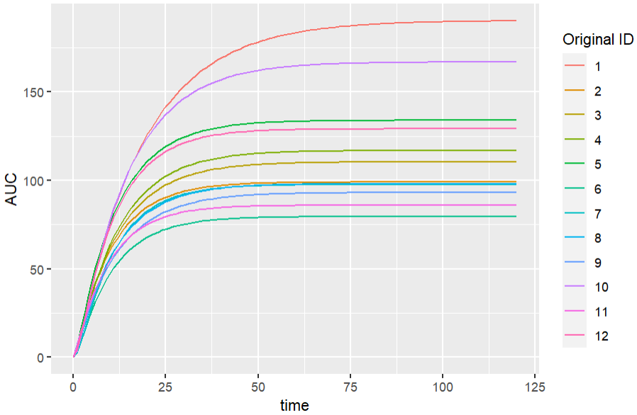
Create a Simulx project from scratch and simulate covariate-dependent treatments
This script creates a project similar to the demo project treatment_weight_and_genotype_based.smlx, available in the folder 3.1.treatments of Simulx demos. The model file TMDDmodel.txt can be downloaded here.
While in the interface of Simulx it is possible to directly define distribution laws for covariates and covariate-dependent treatments that are computed at the simulation step, in R it is necessary to sample covariates from distributions and derive the corresponding doses before defining the elements for the simulation.
###############################################################
# Create a Simulx project from scratch and simulate covariate-dependent treatments
###############################################################

# load and initialize the API
library(lixoftConnectors)
initializeLixoftConnectors(software = "simulx")

# Create a new project based on the model
newProject(modelFile = "TMDDmodel.txt")

# Define vector of population parameters
definePopulationElement(name="PopParameters",
                        element = data.frame(V_pop=3, omega_V=0.1 ,Cl_pop=0.1, omega_Cl=0.1, Q_pop=1, omega_Q=0.2,
                                             V2_pop=3, omega_V2=0.2, beta_V_logtWeight=1, KD_pop=0.01, omega_KD=0.01,
                                             R0_pop=0.2, omega_R0=0.3, kint_pop=50, omega_kint=0.2, kon_pop=10,
                                             omega_kon=0.01, ksyn_pop=10, omega_ksyn=0.2, beta_Cl_logtWeight=0.75,
                                             beta_Q_logtWeight=0.75, beta_V2_logtWeight=0.75,
                                             beta_KD_Genotype_Heterozygous=1.3))

# Define covariates: in the interface it is possible to define distribution laws,
# but in R we have to sample from the distributions prior to the simulation.
# Here we define 3 tables for the 3 simulation groups
for (i in 1:3){
  covTable <- data.frame(id=1:250,
                         Weight = rlnorm(n=250, mean=log(70), sd=0.3),
                         Genotype=c("Homozygous", "Heterozygous")[sample(1:2, 250, replace=T)])
  write.csv(covTable, file = paste0("covTable",i,".csv"), quote=F, row.names=F)
  defineCovariateElement(name=paste0("covTable",i),
                         element = paste0("covTable",i,".csv"))
}

# Define common treatment
defineTreatmentElement(name="1000nmol", element=list(admID=1, data=data.frame(time=seq(0,by=21,length.out = 5),
                                                                              amount=1000, tInf=0.208)))

# Define weight-based treatment: in the interface it can be done directly with a scaling formula,
# but in R we have to define a table of individual doses prior to the simulation.
# We use covTable2.csv for simulation group 2.
covTable <- read.csv("covTable1.csv")
trt_14nmolPerKg <- data.frame(id=rep(1:250, each=5),
                              time=rep(seq(0,by=21,length.out = 5), times=250),
                              amount=14*covTable$Weight, tInf = 0.208)
write.csv(trt_14nmolPerKg, file="trtTableWeight.csv", quote=F, row.names=F)
defineTreatmentElement(name="14nmolPerKg", element=list(admID=1, data="trtTableWeight.csv"))

# Define genotype-based treatment: in the interface it can be done directly with a scaling formula,
# but in R we have to define a table of individual doses prior to the simulation.
# We use covTable3.csv for simulation group 3.
covTable <- read.csv("covTable3.csv")
trt_genotype <- data.frame(id=rep(1:250, each=5),
                           time=rep(seq(0,by=21,length.out = 5), times=250),
                           amount=ifelse(covTable$Genotype=="Heterozygous", 1000, 800), tInf = 0.208)
write.csv(trt_genotype, file="trtTableGenotype.csv", quote=F, row.names=F)
defineTreatmentElement(name="1000nmolHomo_800nmolHetero", element=list(admID=1, data="trtTableGenotype.csv"))

# Define outputs
defineOutputElement(name="Concentration", element = list(output="L", data=data.frame(time=seq(0,96,by=1))))
defineOutputElement(name="TargetOccupancy", element = list(output="TO", data=data.frame(time=seq(0,96,by=1))))

# By default there is a single simulation group named simulationGroup1,
# change its name and set all elements for the simulation
setGroupSize("simulationGroup1", 250)
setGroupElement("simulationGroup1", elements = c("PopParameters","14nmolPerKg","Concentration","TargetOccupancy", "covTable1"))
renameGroup("simulationGroup1", "Weight_based")

# Define the two other simulation groups with different covariates and treatments.
# By default the other elements are the same as the first group
addGroup("Flat_dose")
setGroupElement("Flat_dose", elements = c("1000nmol","covTable2"))
addGroup("Genotype_based")
setGroupElement("Genotype_based", elements = c("1000nmolHomo_800nmolHetero","covTable3"))

# Save project and run the simulation
saveProject(projectFile = "treatment_weight_and_genotype_based.smlx")
runSimulation()

# Get simulation results: a table of individual parameters for each group, and a table of simulated values for each output
sim <- getSimulationResults()
names(sim$IndividualParameters) # "Weight_based", "Flat_dose", "Genotype_based"
names(sim$res) # "L", "TO"
Import a Monolix project and simulate with new output times
Monolix simulates the original dataset with replicates to generate the VPC. It can be useful to perform the same simulations in Simulx with modified observation times, for example to correct the bias in VPC due to dropout. The example below shows this step, and uses the project PDTTE_dropout. The full example to correct a VPC for dropout is detailed on this page.
In this example the Monolix project with the biased VPC is named PD_TTE.mlxtran, the new regular measurement times are similar to the measurements in the original dataset, but are not impacted by dropout, and the number of replicates is 500 (as the default number of simulations for the VPC in Monolix). The random variable capturing dropouts in the model used in Monolix is called survival.
###############################################################
# Import a Monolix project and simulate with new output times
###############################################################

library(lixoftConnectors)
initializeLixoftConnectors(software = "simulx")

importProject(projectFile = "PDTTE_dropout.mlxtran")
defineOutputElement(name="y1_alltimes", element = list(output="y1", data=data.frame(time=seq(-100,1500,by=100))))
setGroupElement("simulationGroup1", elements = c("y1_alltimes","mlx_survival"))
setNbReplicates(500)
saveProject(projectFile = "PD_TTE_alltimes.smlx")
setPreferences(exportsimulationfiles=T)
runSimulation()
Run a simulation with different sample sizes and plot the power of the study based on an endpoint
This piece of code uses the demo project OutcomeEndpoint_PKPD_changeFromBaseline.smlx (demo folder 6.1), with the goal of comparing two treatment arms (400mg Q4W and 800mg Q8W) with a range of different sample sizes (number of simulated individuals per arm). The power of the clinical trial is defined as the chance of having a significant difference in the mean change from baseline between the two arms. This chance is computed over 200 replicates for each sample size. The script then plots the power of the clinical trial with respect to the sample size, with a target power of 85% displayed as a horizontal line.
Note that Simulx versions prior to 2023 did not provide connectors to define the outcomes and endpoints like in the interface.
library(ggplot2)

#initialize LixoftConnectors with Simulx
library(lixoftConnectors)
initializeLixoftConnectors(software="simulx")

# load Simulx demo project comparing 3 treatment arms
project <- paste0(getDemoPath(), "/6.outcome_endpoints/6.1.outcome_endpoints/OutcomeEndpoint_PKPD_changeFromBaseline.smlx") loadProject(projectFile = project) # check the groups defined in the project. # We are interested comparing the two groups 400mg_q4w_ and 800mg_q8w_ for the output "Cholesterol_measured_atCtrough" # -> remove other groups and outputs
getGroups()
removeGroup("400mg_q8w_")
removeGroupElement("400mg_q4w_", "Cholesterol_prediction")
removeGroupElement("800mg_q8w_", "Cholesterol_prediction")
removeGroupElement("400mg_q4w_", "mAbTotal_prediction")
removeGroupElement("800mg_q8w_", "mAbTotal_prediction")

# check the endpoints defined in the project. We are interested in the endpoint mean_changeFromBaseline
getEndpoints()
deleteEndpoint("percentChangeFromBaseline")


#enable group comparison since it is disabled in the demo project
setGroupComparisonSettings(referenceGroup = "400mg_q4w_",enable = TRUE)


# gather endpoints for trials of several sample sizes
Nrep <- 200
sample_sizes <- c(15, 30, 50, 75, 100)
PowerDF = data.frame(sampleSize=sample_sizes,Power=rep(0,length(sample_sizes)))


meanChFromBL <-NULL
for(indexN in 1:length(sample_sizes)){

  N <- sample_sizes[indexN]
  # change the number of individuals for each arm
  setGroupSize("400mg_q4w_", N)
  setGroupSize("800mg_q8w_", N)
  setNbReplicates(Nrep)

  # run the simulation and endpoints
  runScenario()

  # optional - gathering endpoints to plot them for each group and sample size
  meanChFromBL_N <- getEndpointsResults()$endpoints$mean_changeFromBaseline
  meanChFromBL <- rbind(meanChFromBL, cbind(meanChFromBL_N, sampleSize=N))

  # gathering success for each replicate
  successForAllRep <- as.logical(getEndpointsResults()$groupComparison$mean_changeFromBaseline$success)
  PowerDF$Power[indexN]=sum(successForAllRep)/Nrep*100

}

# to plot the results (no connectors available yet for Simulx plots)

library(ggplot2)

ggplot(meanChFromBL, aes(group, arithmeticMean)) +
        geom_boxplot(aes(fill = group)) +
        facet_grid(. ~ sampleSize) +
        ylab("Mean change from baseline at Ctrough")+
        xlab("")+
        theme(axis.text.x = element_blank(), axis.ticks = element_blank())

ggplot(PowerDF)+geom_line(aes(x=sampleSize,y=Power, color="red"))+
  ylab("Power (%)")+xlab("Number of subjects per arm")+geom_hline(yintercept = 85)+
  ylim(c(0,100))+ theme(legend.position = "none")
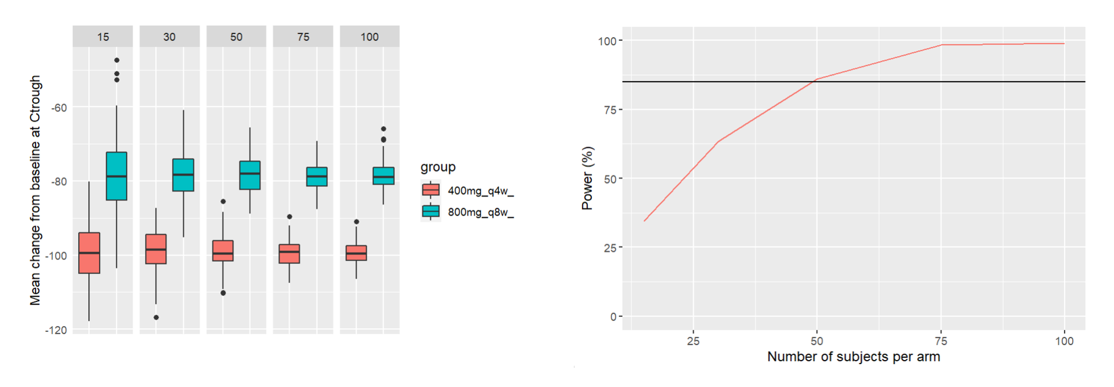
Handling of warning/error/info messages
Error, warning and info messages from Simulx are displayed in the R console when performing actions on a Simulx project. They can be hidden via the R options. Set lixoft_notificationOptions$errors, lixoft_notificationOptions$warnings and lixoft_notificationOptions$info to 1 or 0 to respectively hide or show the messages.
Example
op = options()
op$lixoft_notificationOptions$warnings = 1   #hide the warning messages
options(op)
Force software switch
By default, function initializeLixoftConnectors() prompts users to confirm that they want to proceed with the software switch, in order to avoid losing unsaved changes in the currently loaded project. To override this behavior, force argument can be set to TRUE when calling the function. However, the default behavior can be changed globally as well.
Example
op = options()
op$lixoft_lixoftConnectors_forceSoftwareSwitch <- TRUE
options(op)
6.RsSimulx
RsSimulx is an additional R package which offers two main functionalities:
- provide a wrapper around the lixoftConnectors for Simulx, with a more compact syntax than the lixoftConnectors
- provide a function similar to the simulx() function of the old package mlxR and compatible with the MonolixSuite versions 2020 and 2021, to ease the transition.
Installation
RsSimulx is available on CRAN but it requires the lixoftConnectors package which is provided within the MonolixSuite installation. In addition RJSONIO (available on CRAN) is required.
Installation of RJSONIO (from CRAN)
install.packages("RJSONIO")
Installation of the lixoftConnectors
The lixoftConnectors are not available on CRAN. The installation package is located in the MonolixSuite installation directory. The default path to the installation directory differs between operating systems. You may have to adapt the path if you have chosen another installation directory.
# for Windows install.packages("C:/ProgramData/Lixoft/MonolixSuite2023R1/connectors/lixoftConnectors.tar.gz", repos = NULL, type="source",INSTALL_opts ="--no-multiarch")# for MAC OS install.packages("/Applications/MonolixSuite2023R1.app/Contents/Resources/monolixSuite/connectors/lixoftConnectors.tar.gz", repos = NULL, type="source", INSTALL_opts ="--no-multiarch") # for Linux install.packages("/home/<your username>/Lixoft/MonolixSuite2023R1/connectors/lixoftConnectors.tar.gz", repos = NULL, type="source", INSTALL_opts ="--no-multiarch")
Installation of RsSimulx
install.packages("RsSimulx", INSTALL_opts ="--no-multiarch")Change log
Version 2023.1 (released on CRAN on April 20th 2023)
This version is compatible with MonolixSuite version 2023. The lixoftConnectors 2023 should be installed first.
- In case of simulations using elements defined via external files, output will contain a column “original_id” indicating id of individuals in external files.
- Versioning was changed to be consistent with lixoftConnectors and MonolixSuite versioning.
Version 2.0.0 (released on CRAN on February 18th 2022)
This version is compatible with MonolixSuite version 2021. The lixoftConnectors 2021 should be installed first.
In this version, new functionalities already available in the GUI were added and the syntax has been slightly changed to be consistent with the display in the GUI.
The main changes in the simulx() function are summarized below:
- parameter:
- accept only pop param and indiv param (and ‘remaining parameters’). No covariates anymore, use the “covariate” argument instead.
- accept strings corresponding to the elements automatically generated after an import:”mlx_Pop”, “mlx_PopUncertainSA”, “mlx_PopUncertainLin”, “mlx_PopIndiv”, “mlx_PopIndivCov”,”mlx_CondMean”,”mlx_EBEs”,”mlx_CondDistSample”
- deprecated: “mode” and “mean” (use the keyword above instead)
- covariate:
- accepts covariates elements as lists (same value for all individuals), data frames or path to text file
- accept strings corresponding to the elements automatically generated after an import: “mlx_Cov” and “mlx_CovDist”
- treatment:
- accept string corresponding to the elements automatically generated after an import: “mlx_admXXX”
- new options “repeats” and “probaMissDose”
- varlevel:
- deprecated and now called “occasion”
- nrep:
- now samples with or without uncertainty depending which element is given as “parameter”
- stat.f, data, result_folder et les settings load.design, data.in, disp.iter:
- have been removed
- npop and fim:
- deprecated: use nrep and “mlx_PopUncertainSA” or “mlx_PopUncertainLin” instead
- settings:
- “kw.max”: deprecated
- “replacement”: has been replaced by “samplingMethod” with values “keepOrder”, “withReplacement”, “withoutReplacement”
- new option “sameIndividualsAmongGroups”: true/false
- new option “sharedIds”: vector of strings among covariate, output, treatment, regressor, population, individual.
- new option “exportData”: true/false
- saveSmlxProject:
- save the .smlx project to the specified path.
Known limitations:
- when just resimulating a Monolix project, the individuals having no observations for some obs ids (in case of several observation identifiers) or no dose will be missing from the simulation.
- it is not possible to retrieve the original IDs when using data frames with id column as input
Version 1.0.1 (released on CRAN on April 8th 2021)
This version corrects several bugs and is compatible with MonolixSuite version 2020.
- The initialization of the lixoftConnectors (i.e linking to the MonolixSuite installation folder) is now done on the first call to simulx() instead of the loading of the RsSimulx package.
- The new function initRsSimulx(path=…) allows to indicate a path to the MonolixSuite installation folder when the <home>/lixoft/lixoft.ini file is missing or needs to be bypassed.
- Messages, warnings and errors raised by the lixoftConnectors are now propagated to RsSimulx such that the user can see them.
- Columns “type” or “adm” for treatments defined as data.frames are now properly recognized (they where previously ignored).
- When both population parameters and covariates are given in the “parameter=” argument of simulx(), the covariates are now properly taken into account (they were previously ignored).
- The seed given to simulx() now propagates to simpopmlx, which is sampling the population parameters when using the argument “npop” (previously the reproducibility was not ensured when using npop).
- The use of a named vector with only characters (typically in the case of categorical-only covariates defined as strings) does not generate an error any more.
-
When population parameters are defined as a data.frame with a column “pop”, the dataframe is now used with the correct number of rows (it was previously cut or replicated to match the npop argument).
- When npop is used but no treatment is present, no error is raised anymore.
- When the “parameter” argument is defined as a named vector with both characters (for categorical covariates for instance) and numerical values, no error is raised anymore.
Known issues remaining in version 1.0.1:
- regressor values are not outputted from simulx()
- when just resimulating a Monolix project, in case of both continuous and non-continuous outputs, only the continuous outputs are outputted.
Version 1.0.0 (released on CRAN on January 21st 2021)
RsSimulx is compatible with the MonolixSuite version 2020. It provides retro-compatibility of old mlxR scripts and functions to complement the use of Simulx-GUI (writeData(), prctilemlx() and simpopmlx()).
6.1.RsSimulx usage
- simulx() to run the simulation
- prctilemlx() to plot prediction intervals (with overlay of the groups on a single plot)
- writeData() to write the simulation results to a MonolixSuite compatible format – This feature is now available directly in the interface and in the API with exportSimulatedData.
prctilemlx(): prediction interval plots
Description
Compute and plot percentiles of the empiricial distribution of longitudinal data. When several groups are present, the groups can be plotted as subplots or as different colors on one plot. The input can be a R object (parameter r) or a monolix project and a variable name (arguments project and outputVariableName).
Usage
prctilemlx(
  r = NULL,
  col = NULL,
  project = NULL,
  outputVariableName = NULL,
  number = 8,
  level = 80,
  plot = TRUE,
  color = NULL,
  group = NULL,
  facet = TRUE,
  labels = NULL,
  band = NULL
)
Arguments
r |
a data frame with a column id, a column time and a column with values. The times should be the same for all individuals. |
col |
a vector with the three column indexes for id, time and y. Default = c(1,2,3). |
project |
simulx project filename (with extension “.smlx”) |
outputVariableName |
name of the output to consider. By default the first output will be consider. You must define either a ‘r’ dataframe (and the associated ‘col’ argument) or a simulx project and the name of the output ‘outputVariableName” |
number |
the number of intervals (i.e. the number of percentiles minus 1). |
level |
the largest interval (i.e. the difference between the lowest and the highest percentile). |
plot |
if TRUE the empirical distribution is displayed, if FALSE the values are returned |
color |
colors to be used for the plots In case of one group or facet = TRUE, only the first color will be used |
group |
variable to be used for defining groups (by default, ‘group’ is used when it exists) |
facet |
makes subplots for different groups if TRUE |
labels |
vector of strings |
band |
is deprecated (use number and level instead) ; a list with two fields
|
Details
You must define either a dataframe r (and if needed the associated col argument) or a simulx project and the name of the output outputVariableName. The outputVariableName corresponds to the name of the model variable, not to the output element name.
Value
a ggplot object if plot=TRUE ; otherwise, a list with fields:
- proba: a vector of probabilities of length
band$number+1 - color: a vector of colors used for the plot of length
band$number - y: a data frame with the values of the empirical percentiles computed at each time point
Examples
This simulx-GUI demo project contains 3 simulation groups, with a low, medium or high dose. In the Simulation tab, the output element ‘regularCc’ is selected, to output the variable ‘Cc’ on a regular time grid.
With facet=T (default), each group is displayed on a separate subplot with the different shades representing different percentiles. The largest band represents the 90% prediction interval.
project.file <- "~/../lixoft/simulx/simulx2020R1/demos/5.simulation/simulationGroups_treatment.smlx"
prctilemlx(project=project.file, outputVariableName = "Cc")
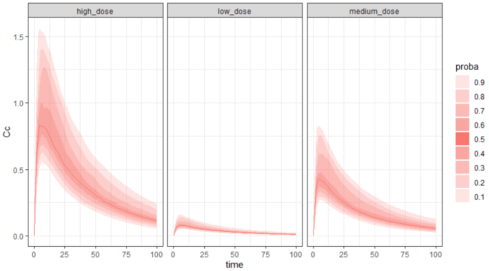
With number=2 and level=95, we can select to display only the median and the 95% prediction interval.
project.file <- "~/../lixoft/simulx/simulx2020R1/demos/5.simulation/simulationGroups_treatment.smlx"
prctilemlx(project=project.file, outputVariableName = "Cc", number=2, level=95)
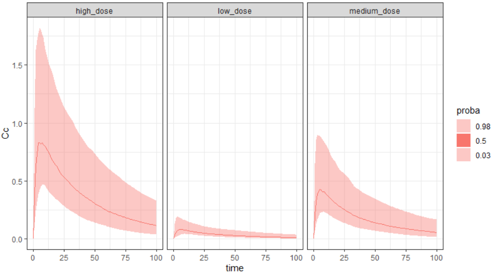
To display the prediction intervals on top of each other, use facet=F. As a ggplot object is returned, additional ggplot functions can be used to overlay additional features or modify the legend, etc.
prctilemlx(project=project.file, outputVariableName = "Cc", facet=F, number=2, level=95) + ylab("Concentration (ug/mL)") + xlab("Time (hr)") + geom_hline(yintercept = 0.25)
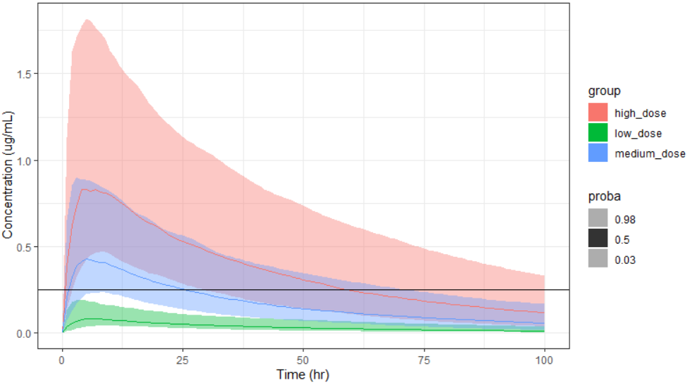
See also http://simulx.webpopix.org/mlxr/prctilemlx/ for more examples.
- simulx() to run the simulation [documentation under construction]
- writeData() to write the simulation results to a MonolixSuite compatible format
- prctilemlx() to plot prediction intervals (with overlay of the groups on a single plot)
writeData(): write simulations to MonolixSuite data set format
Description
Format outputs of simulx simulations and write datasets in monolix and pkanalix project format.
Usage
writeData(
  project = NULL,
  filename = "simulated_dataset.csv",
  sep = ",",
  ext = "csv",
  nbdigits = 5
)
Arguments
project |
(string) a simulx project with extension .smlx. If no project is specified, the function will run on the project that is already loaded. |
filename |
(string) (optional) file path to dataset. (default “simulated_dataset.csv”) In case of multiple replicates, the function creates one dataset per replicate with name $filename_repi If filename contains an extension, it must be “csv” or “txt”. If it does not, extension is defined by ext argument. |
sep |
(string) (optional) Separator used to write dataset file. (default “,”) It must be one of “\t”, ” “, “;”, “,” |
ext |
(bool) (optional) Extension used to write dataset file. (default “csv”) It must be one of “csv”, “txt” To defined only if filename with no extension |
nbdigits |
(integer) (optional) number of decimal digits in output file. (default = 5) |
Details
The generated data set has the following headers: id, occ (if occasions have been used), time, amt, adm, rate, y (observations), ytype (observation id), evid (if a washout was defined), and the covariates names.
WARNING: writeData function is not implemented for simulx project with regressors in MonolixSuite version 2020R1. When a loq is defined in the simulx() function, it is not taken into account when writing the data set.
Value
a dataframe if one single simulation, a list of dataframes if multiple replicates.
Examples
The Simulx-GUI demo simulates a PK/PD data set. The saved data set has the standard format to be loaded in Monolix or Simulx.
project.file <- "~/../lixoft/simulx/simulx2020R1/demos/1.overview/importFromMonolix_resimulateProject.smlx"
writeData(project=project.file, filename = "simdata.csv")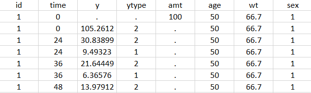
prctilemlx(): prediction interval plots
Description
Compute and plot percentiles of the empiricial distribution of longitudinal data. When several groups are present, the groups can be plotted as subplots or as different colors on one plot. The input can be a R object (parameter r) or a monolix project and a variable name (arguments project and outputVariableName).
Usage
prctilemlx(
  r = NULL,
  col = NULL,
  project = NULL,
  outputVariableName = NULL,
  number = 8,
  level = 80,
  plot = TRUE,
  color = NULL,
  group = NULL,
  facet = TRUE,
  labels = NULL,
  band = NULL
)
Arguments
r |
a data frame with a column id, a column time and a column with values. The times should be the same for all individuals. |
col |
a vector with the three column indexes for id, time and y. Default = c(1,2,3). |
project |
simulx project filename (with extension “.smlx”) |
outputVariableName |
name of the output to consider. By default the first output will be consider. You must define either a ‘r’ dataframe (and the associated ‘col’ argument) or a simulx project and the name of the output ‘outputVariableName” |
number |
the number of intervals (i.e. the number of percentiles minus 1). |
level |
the largest interval (i.e. the difference between the lowest and the highest percentile). |
plot |
if TRUE the empirical distribution is displayed, if FALSE the values are returned |
color |
colors to be used for the plots In case of one group or facet = TRUE, only the first color will be used |
group |
variable to be used for defining groups (by default, ‘group’ is used when it exists) |
facet |
makes subplots for different groups if TRUE |
labels |
vector of strings |
band |
is deprecated (use number and level instead) ; a list with two fields
|
Details
You must define either a dataframe r (and if needed the associated col argument) or a simulx project and the name of the output outputVariableName. The outputVariableName corresponds to the name of the model variable, not to the output element name.
Value
a ggplot object if plot=TRUE ; otherwise, a list with fields:
- proba: a vector of probabilities of length
band$number+1 - color: a vector of colors used for the plot of length
band$number - y: a data frame with the values of the empirical percentiles computed at each time point
Examples
This simulx-GUI demo project contains 3 simulation groups, with a low, medium or high dose. In the Simulation tab, the output element ‘regularCc’ is selected, to output the variable ‘Cc’ on a regular time grid.
With facet=T (default), each group is displayed on a separate subplot with the different shades representing different percentiles. The largest band represents the 90% prediction interval.
project.file <- "~/../lixoft/simulx/simulx2020R1/demos/5.simulation/simulationGroups_treatment.smlx"
prctilemlx(project=project.file, outputVariableName = "Cc")
With number=2 and level=95, we can select to display only the median and the 95% prediction interval.
project.file <- "~/../lixoft/simulx/simulx2020R1/demos/5.simulation/simulationGroups_treatment.smlx"
prctilemlx(project=project.file, outputVariableName = "Cc", number=2, level=95)
To display the prediction intervals on top of each other, use facet=F. As a ggplot object is returned, additional ggplot functions can be used to overlay additional features or modify the legend, etc.
prctilemlx(project=project.file, outputVariableName = "Cc", facet=F, number=2, level=95) + ylab("Concentration (ug/mL)") + xlab("Time (hr)") + geom_hline(yintercept = 0.25)
See also http://simulx.webpopix.org/mlxr/prctilemlx/ for more examples.
writeData(): write simulations to MonolixSuite data set format
Description
Format outputs of simulx simulations and write datasets in monolix and pkanalix project format.
Usage
writeData(
  project = NULL,
  filename = "simulated_dataset.csv",
  sep = ",",
  ext = "csv",
  nbdigits = 5
)
Arguments
project |
(string) a simulx project with extension .smlx. If no project is specified, the function will run on the project that is already loaded. |
filename |
(string) (optional) file path to dataset. (default “simulated_dataset.csv”) In case of multiple replicates, the function creates one dataset per replicate with name $filename_repi If filename contains an extension, it must be “csv” or “txt”. If it does not, extension is defined by ext argument. |
sep |
(string) (optional) Separator used to write dataset file. (default “,”) It must be one of “\t”, ” “, “;”, “,” |
ext |
(bool) (optional) Extension used to write dataset file. (default “csv”) It must be one of “csv”, “txt” To defined only if filename with no extension |
nbdigits |
(integer) (optional) number of decimal digits in output file. (default = 5) |
Details
The generated data set has the following headers: id, occ (if occasions have been used), time, amt, adm, rate, y (observations), ytype (observation id), evid (if a washout was defined), and the covariates names.
WARNING: writeData function is not implemented for simulx project with regressors in MonolixSuite version 2020R1. When a loq is defined in the simulx() function, it is not taken into account when writing the data set.
Value
a dataframe if one single simulation, a list of dataframes if multiple replicates.
Examples
The Simulx-GUI demo simulates a PK/PD data set. The saved data set has the standard format to be loaded in Monolix or Simulx.
project.file <- "~/../lixoft/simulx/simulx2020R1/demos/1.overview/importFromMonolix_resimulateProject.smlx"
writeData(project=project.file, filename = "simdata.csv")
6.2.RsSimulx simulx() function
simulx(): simulation of mixed effects models and longitudinal data
Description
Compute predictions and sample data from Mlxtran and R models
Usage
simulx(
  model = NULL,
  parameter = NULL,
  covariate = NULL,
  output = NULL,
  treatment = NULL,
  regressor = NULL,
  occasion = NULL,
  varlevel = NULL,
  group = NULL,
  project = NULL,
  nrep = 1,
  npop = NULL,
  fim = NULL,
  saveSmlxProject = NULL,
  result.file = NULL,
  addlines = NULL,
  settings = NULL
)
Arguments
model |
(string) a Mlxtran model used for the simulation. It can be a text file or an output of the inLine function. |
parameter |
One of
|
covariate |
One of
|
output |
output or list of outputs. An output can be defined by
|
treatment |
treatment or list of treatments. A treatment can be defined by
|
regressor |
treatment or list of treatments. A treatment can be defined by
|
occasion |
An occasion can be defined by
|
varlevel |
deprecated, use occasion instead. |
group |
a list, or a list of lists, with fields:
“level” field is not supported anymore in RsSimulx. |
project |
the name of a Monolix project |
nrep |
Samples with or without uncertainty depending which element is given as “parameter”. |
npop |
deprecated, set parameter = “mlx_popUncertainSA” or “mlx_popUncertainLin” instead. |
fim |
deprecated, set parameter = “mlx_popUncertainSA” or “mlx_popUncertainLin” instead. |
saveSmlxProject |
If specified, smlx project will be save in th path location (by default smlx project is not saved) |
result.file |
deprecated |
addlines |
a list with fields:
“section”, “block” field are not supported anymore in RsSimulx. You only need to specify a formula. The additional lines will be added in a new section EQUATION. |
settings |
a list of optional settings
|
Details
simulx takes advantage of the modularity of hierarchical models for simulating different components of a model: models for population parameters, individual covariates, individual parameters and longitudinal data.
Furthermore, simulx allows to draw different types of longitudinal data, including continuous, count, categorical, and time-to-event data.
The models are encoded using either the model coding language Mlxtran. Mlxtran models are automatically converted into C++ codes, compiled on the fly and linked to R using the RJSONIO package. That allows one to implement very easily complex models and to take advantage of the numerical sovers used by the C++ mlxLibrary.
Value
A list of data frames. Each data frame is an output of Simulx
Examples
Example 1: simulation from scratch
This example shows how to create a Simulation from scratch and plot the results.
myModel <- inlineModel("
  [LONGITUDINAL]
  input = {A, k, c, a}
  EQUATION:
  t0 = 0
  f_0 = A
  ddt_f = -k*f/(c+f)
  DEFINITION:
  y = {distribution=normal, prediction=f, sd=a}
  [INDIVIDUAL]
  input = {k_pop, omega}
  DEFINITION:
  k = {distribution=lognormal, prediction=k_pop, sd=omega}
")

f <- list(name='f', time=seq(0, 30, by=0.1))
y <- list(name='y', time=seq(0, 30, by=2))
parameter <- c(A=100, k_pop=6, omega=0.3, c=10, a=2)

res <- simulx(model = myModel,
parameter = parameter,
occasion = data.frame(time=c(0, 0), occ=c(1, 2)),
output = list(f,y),
group = list(size=4),
saveSmlxProject = "./project.smlx")

res <- simulx(model = myModel,
parameter = parameter,
occasion = data.frame(time = c(0, 0, 0, 0),
occ1 = c(1, 1, 2, 2),
occ2 = c(1, 2, 3, 4)),
output = list(f,y),
group = list(size=4))

res <- simulx(model = myModel,
parameter = parameter,
output = list(f,y),
group = list(size=4))

plot(ggplotmlx() + geom_line(data=res$f, aes(x=time, y=f, colour=id)) +
geom_point(data=res$y, aes(x=time, y=y, colour=id)))
print(res$parameter)
Example 2: simulation from a Monolix project
This example shows how to simulate from a Monolix project (using a Monolix demo): first with all the simulation elements exported from Monolix (Simulx resimulates the dataset from Monolix using the population parameter estimated in the Monolix project), then with a new design for the treatment (4 doses are given to all individuals), output (Cc is recorded instead of CONC, so the residual error is not included in the simulations) and group size (20 simulated individuals).
# First use the Monolix connectors to get the path to the demos and estimate the population parameters of the Monolix project
library(lixoftConnectors)
initializeLixoftConnectors(software = "monolix")
demoProject <- paste0(getDemoPath(),"/1.creating_and_using_models/1.1.libraries_of_models/theophylline_project.mlxtran")
loadProject(demoProject)
runPopulationParameterEstimation()

# Then use RsSimulx for the simulations
library(RsSimulx)

res <- simulx(project = demoProject)
plot(ggplotmlx() + geom_line(data=res$CONC, aes(x=time, y=CONC, colour=id)) +
geom_point(data=res$CONC, aes(x=time, y=CONC, colour=id)))

res <- simulx(project = demoProject,
              treatment = list(time=seq(0, by=24,length=4), amount=4),
              group = list(size=20),
              output = list(name="Cc", time=1:120))

prctilemlx(res$Cc)

6.3.RsSimulx for retrocompatibility of mlxR scripts
RsSimulx contains a function simulx() which works in the same way as the simulx() function of the mlxR package. To use your scripts initially developed with mlxR with MonolixSuite 2020, 2021 and 2023, you need to replace library(mlxR) by library(RsSimulx) and run the rest of your script as before.
Removed features
A few functions and features which were available in the mlxR package are not available in the RsSimulx package anymore, due to technical constrains. They are listed below.
- the following functions have been removed:
- pkmodel()
- monolix2simulx()
- readDataMlx()
- the following arguments have been removed from the simulx() function
- in “treatment=”, the “target” field is not accepted anymore. Use “adm” instead.
- in “group=”, the “level” field is not accepted anymore, unless it is equal to “individual”. With RsSimulx, the variability is always at the individual level.
- The following outputs have been removed:
- originalID data frame (but originalID is now part of result tables returned by getSimulationResults() in tables of individual parameters and outputs next to the ID column, and as a separate table ID_mapping if external elements have been used)
Modifications requiring small code adaptations
- the individual parameters are covariates are now outputted by default in the ‘parameter’ argument. It is not necessary to request them explicitly.
- the writeDataMlx() function has been replaced by the function exportsimulatedData() which is called without R object as input. When called just after a simulx() call, it will use the simulx project in memory to write the data set. Note that the ‘loq’ will not be taken into account.
- overlapping occasions are now supported but when the occasion element has an id column, all elements must follow this occasions structure. See the occasion definition in Simulx-GUI for more details.
- for time-to-event outputs, it is now required to give a vector of two times (start and end of the observation period) instead of only the start time:
out <- list(name="Event", time=c(0, 400)) - Negative amount with positive infusion rates are not possible anymore. Use the reset or empty macros instead.
- it is not possible to define distributions in the [COVARIATE] or [POPULATION] block anymore. Instead, sample the covariates or population parameters in the R script and provide them as a data frame.
- in the model, to properly identify covariates, individual parameters and population parameters, they must be declared in the corresponding block. The model structure is detailed on the mlxtran page.
Reproducibility
Running the same script with RsSimulx or mlxR will lead to different simulated values because the seed is read in a different way by the two packages. When running the same script several times with RsSimulx, the simulated values will be the same.
6.4.mlxR documentation
The legacy documentation for the mlxR package can be downloaded from here. The documentation contains user guides for the package functions, as well as multiple case studies and R scripts.
7.Case studies
The case studies below show how to use Simulx for simulations.
Setting up a simulation from scratch
You can start a Simulx project by importing a Monolix run or you can define every element needed for the simulation from scratch. In this webinar, we explain how to setup a simulation by defining the model, parameters, treatments and outputs. A special focus will be given on the model writing in mlxtran language, with examples of translations from Nonmem and literature models.
The slides explain how to define each part of the mlxtran model and show screenshots of how to define the elements for the simulation in the GUI. The key points and results are also on the slides. The webinar can be reproduced step-by-step using the provided Simulx projects.
From Monolix to Simulx: how to explore new scenarios
When you have built a model, you can use it to compare new dosing regimens for the next trial, calculate the expected power of a study and select the most successful strategy? Learn effortless exploration of new scenarios with Simulx GUI – intuitive, flexible, and powerful application to simulate and compare countless strategies – and switch your focus to analysis and decision-making.
This video explains using Simulx with Monolix projects, it shows step-by-step how to simulate different groups, define target outcomes and assess the uncertainty and presents features that bring the best insight from simulations.
Optimizing Sample Size of a Phase III Trial
What if we could reduce the size of a phase III study from 400 to 80 subjects and make it twice as short? Thanks to model-informed clinical trial design, it’s possible! Watch an inspiring story based on real-world case study data and learn about Simulx at the same time. In an hour, we will take you from the modeling of phase II studies in Monolix to the estimation of a phase III study power in Simulx to finally optimizing sample size and study duration. Example scripts to script Simulx from R as done in this webinar can be found here.
8.Frequently asked questions
- Download, Installation, Run and Display issues
- General questions
- Model
- Definition tab
- Exploration tab
- Simulation tab
- Results and Outputs
- Plots
- LixoftConnectors
- Share your Feedback
GENERAL
- How can I reuse my previous mlxR scripts (which where using the simulx() R function)?
Simulx has evolved a lot between the 2019 and 2020 versions, and its API also. mlxR (and its simulx() function) is not compatible with Simulx versions starting from 2020.However Simulx 2020 is available via a very convenient and intuitive GUI, and via a complete R API, which allows to do from R any step that exists in the GUI.To make the transition smoother, we also provide an additional R package RsSimulx with a simulx() wrapper function using the R API, very similar to the simulx() function of mlxR. All deprecated arguments coming from the mlxR syntax will generate a warning with RsSimulx versions starting from 2.0.0.
- It is possible to automatically convert a Nonmem model to a Simulx model? No, but the conversion is relatively easy. For the structural model, you can replace the Nonmem ADVAN routines 1-3 by the pkmodel macro, and the syntax for ODEs is easy to adapt. Parameter distributions and covariate effects are defined in the [INDIVIDUAL] section.
You can also check our case studies (video and slides) “Setting up a simulation from scratch” will gives examples of translations from Nonmem to Simulx. - How can I share a Simulx project? A Simulx project is composed of a .smlx file, possibly external files you have used to define elements (model file, covariate table, etc) and a result folder. All these must be shared, keeping the relative path between them. In the Simulx project settings (Settings > Project settings > “Save the user files in the results folder”), you can request to save the external files (model and other input files) in the result folder. This way, you only need to share the .smlx file and the result folder.
- How fast is Simulx? Simulx is very fast because it performs the calculations using a C++ engine (the same as Monolix).
- Is it possible to script my simulations? Yes. All actions done in the GUI can also be done via R functions. Have a look at the lixoftConnectors.
MODEL
- Do I have to define correlations between all parameters (i.e full omega matrix)? No. The omega matrix need to be block diagonal only. See the correlation definition here.
DEFINITION tab
- Is it possible to include uncertainty of the population parameters? Yes. If you have obtained sets of population parameters via bootstrap, you can define the population parameter element via an external file with several lines, each line corresponding to a different set of population parameters. You can also define the population parameters using the type “distribution” which will allow to sample the population distribution from an uncertainty distribution. You can for instance choose normal distributions and give the estimated standard errors in the “sd” column. However this does not include correlations between estimates. To include those, you need to sample to population parameters from their uncertainty distribution outside Simulx and provide them as external file. We will provide soon a R package Rssimulx to help for this.
Note that the a different of population parameters will be used for each replicate. - Is it possible to sample covariates from a truncated normal distribution? Not yet. For the moment you can use a logit distribution if you need bounds, or sample the covariate elsewhere and provide an external file.
- Can I flexibly define a treatment depending on covariates (such as WT or BSA)? Yes, this is possible if you have the covariate appearing in your model. Select “scale amount by a covariate” in the treatment definition.
EXPLORATION tab
no question yet
SIMULATION tab
- Can we perform trial simulations accounting for drop-outs? You can define a joint model with PD and a time-to-event model representing the drop-outs. Simulx will simulate the time of drop-out, but not remove observations happening after the drop-out. This will request to post-process the results outside Simulx.
- Can I calculate the time of Cmax? This can be done in the outcome definition. Select the output corresponding to the concentration, then “max per id” and “time of max”.
RESULTS and OUTPUTS
- How can I get the simulated values? The population parameters, individual parameters, doses, covariates and regressors are saved as .txt files in the Simulation folder of the result folder. By default the simulated values are not exported because they can be very large in size. However it is possible to choose this option in Settings > Preferences > Export simulation files. Outcomes and endpoints are saved in the Endpoints folder of the results.
You can also get the results using the lixoftConnectors R package. - What is the best way to post-process the Simulx results in R? You can use the R package lixoftConnectors to interact with your Simulx run. In particular, the function getSimulationResults() allows you to recover all results. These results can then be post-processed using typical R code.
PLOTS
- Is it possible to display a 90% prediction interval? Yes, by default the different shades of blue in the “Output distribution” plot represent different percentiles. If in the “Display” settings in the right panel you choose band=2 and level=90, then you will see a 90% prediction interval.
LIXOFTCONNECTORS
- setGroupElement() worked in 2021R1 but gives an error in the 2021R2 version. The error message has been added in the R2 version when potentially incompatible elements are set together, eg. parameters as EBEs and covariates. In this case you need to set each element separately, as the error message suggests.
- getSimulationResults() does not return results It can happen if the results are too large (too many data points). In the 2021R2 version there are additional two arguments, ID and REP, to request a subset of results.
SHARE YOUR FEEDBACK
- I would like to give a suggestion for the future versions of Simulx. Share your feedback!
- I need more details in the documentation for a specific feature. Share your feedback!
8.1.List of known bugs
The list of known bugs in every version of MonolixSuite can be found in the release notes of the next version.
- Release Notes for MonolixSuite2023R1
- Release Notes for MonolixSuite2021R2
- Release Notes for MonolixSuite2021R1
- Release Notes for MonolixSuite2020R1
We list below the known bugs in Simulx 2023R1 (they will be fixed in the next version). The 2023R1 version of MonolixSuite can be downloaded here.
Installation
- The lixoft folder inside temp is not deleted after installation.
Documentation
- In the Documentation tab, the tutorials section can be empty (due to issues with the host server).
Export simulated data
- Simulated data gets exported to the default location when clicking Cancel in the pop-up window.
Export from/to Monolix
- During export from Monolix to Simulx, parameters with different case (eg “Par” and “par”) were considered the same for individual parameters.
- Exporting a Simulx project to Monolix leads to an error if individual parameters in the structural model input={} line are listed on several lines.
